

Cross-asset correlations in a more inflationary environment and challenges for diversification strategies
Published as part of the Financial Stability Review, November 2022.
Investors can reduce portfolio risk by combining assets that are not perfectly correlated. Diversification is a key ingredient in the asset allocation process under portfolio theory, as idiosyncratic risk can be lowered by combining assets or asset classes that are not perfectly correlated. Historically, stocks and bonds have tended to show a low positive (< 0.5) or even negative correlation of returns (Chart A). The classic “60/40 split” of stocks and bonds, often seen as a benchmark for passive investors, is an example of a portfolio that attempts to provide a better risk-adjusted return by adding bonds to a pure equity portfolio.[1] Although returns on bonds are typically lower than those on equities over longer spans of time, their diversification benefits justify the inclusion of bonds in a portfolio.
The correlation between stock and bond returns has increased recently (Chart A, panel a).[2] Correlations between stock and bond returns tended to be positive between the late 1960s and the late 1990s but turned negative during the 2000s (Chart A, panel b). Various explanations have been proposed for this shift. Some argue that in the presence of supply shocks, real output and inflation tend to move in opposite directions, as was seen during the 1970s and 1980s.[3] As bond coupons are fixed, higher expected inflation should have a negative impact on bond returns. Lower expected output would, under the scenario of an adverse supply shock, negatively affect expected dividends and, therefore, stock returns. Following this logic, supply shocks could result in more correlated stock and bond returns.
Chart A
The stock-bond correlation has increased recently in the euro area and the United States
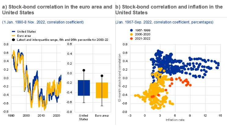
Sources: Refinitiv and ECB calculations.
Notes: Panel a: the stock-bond correlation is computed based on a twelve-month moving window and stock and bond returns at a daily frequency. For the euro area, the ten-year German government bond yield is used to capture bond returns; the EURO STOXX index is used for equity (total) returns. Panel a and panel b: US bond returns are based on ten-year US Treasury yields; equity returns are based on total returns for the S&P 500 Composite index.
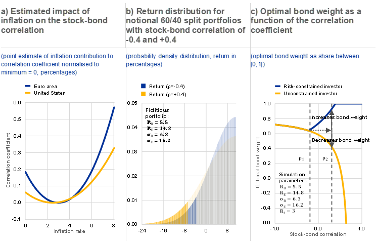
The recent increase in the stock-bond correlation might be related to inflationary pressures, according to an empirical analysis for the United States and the euro area which accounts for the impact of inflation, output growth and changes in risk appetite. Inflation may affect stock and bond returns through different channels, most notably the discount rate channel. When inflation deviates substantially from the central bank’s target, market participants tend to anticipate the impact of policy tightening or expansion. This affects discount rates which may, in turn, affect asset prices across the board, potentially leading to co-movement across asset classes and higher cross-asset correlations.[4] Inflation may also have an asymmetric impact on stocks and bonds because future dividends may increase with prices while fixed coupon payments on bonds do not adjust for inflation. Empirical evidence suggests that the contribution of inflation to the stock-bond correlation could be non-linear. All else equal, the correlation seems to be lowest in both the euro area and the United States when inflation is close to 2% (Chart B, panel a). This could be related to the role of monetary policy expectations, as these might be more important when inflation is significantly above or below the central bank’s target rate. These findings suggest that the recent increase in the stock-bond correlation may be related to elevated inflationary pressures and monetary policy tightening.
Chart B
A higher stock-bond correlation may be linked to higher inflation and could lead to an underestimation of the magnitude and frequency of losses, as well as a higher concentration of risk
Sources: Refinitiv and ECB calculations.
Notes: Panel a: the model used builds on Andersson et al.* In line with this paper, risk appetite (or “flight-to-safety behaviour”) is proxied by the VSTOXX. A decline in risk appetite (increase in VSTOXX) is found to be associated with a lower stock-bond correlation. Instead of GDP, consumer confidence is included to proxy real growth dynamics. In addition, the inflation rate is included both linearly and quadratically, allowing non-linear dynamics to be captured. The empirical analysis is based on monthly data. The model uses simple (robust) Ordinary Least Squares (OLS) estimators and maps the regressors to the interval [-1,1] by means of an adjusted sigmoid function similar to that in Andersson et al., where The parameter estimates and their standard errors for and are given by -0.283 with standard error of 0.062 and with standard error of 0.009 for the euro area. Estimates are based on monthly data from 1 January 2000 to 30 September 2022. Panels b and c: parameters are given as percentages, where and stand for stock return and volatility, and and for bond return and volatility. stands for the risk-free rate. Panel c: risk-constrained investors are required to limit their maximum expected portfolio return volatility to . Both investor types (constrained and non-constrained) optimise their expected risk-adjusted return, defined as the ratio of the portfolio’s excess return to volatility. A number of assumptions have been made for the parameter values but, in qualitative terms, the main results of the simulation presented hold for a wide range of parameters.
*) Andersson, M., Krylova, E. and Vähämaa, S., “Why Does the Correlation between Stock and Bond Returns Vary Over Time?”, Applied Financial Economics, Vol. 18, Issue 2, 2008, pp. 139-151.
A higher correlation between stock and bond returns might lead to an initial underestimation of portfolio risk, increasing the risk of an abrupt adjustment later. Strategic asset allocations and risk models are often calibrated on historical return distributions, but these may not be representative for volatile market conditions.[5] Specifically, if cross-asset correlations increase, total portfolio risk and resulting losses may be larger or more frequent than expected (Chart B, panel b). This may lead investors to rebalance more frequently in response to hitting risk limits which could, in turn, contribute to higher market volatility. And a recent survey of institutional investors suggests that unstable cross-asset correlations are indeed a major current concern for multi-asset portfolios.[6]
Portfolio adjustments in response to higher cross-asset correlations could lead to a larger concentration of risk among certain market participants. Market participants may adjust their portfolios in the face of changing cross-asset correlations. For a portfolio consisting of equities and bonds, an investor that optimises their risk-adjusted return[7] would allocate a smaller (or even negative) share of their wealth to bonds when stock-bond correlations are higher. This is because the relatively limited diversification benefits no longer justify the inclusion of lower yielding bonds in the portfolio (Chart B, panel c). Such portfolio rebalancing flows may add to upward pressures on bond yields. An investor that is subject to a risk constraint, however, might need to increase bond holdings to remain compliant with their investment mandate. In other words, risky-asset holdings (in this case equities) could be concentrated in a smaller subset of market participants that are subject to fewer or lower risk constraints.
The 60/40-split portfolio is often used as a reference portfolio in the investment industry, and a starting point for an initial asset allocation. It is also an important component of the “Norway Model”, which is considered one the major investment strategies for sovereign wealth funds.
Different types of correlation coefficient can be computed. For example, the length of the relevant time window should be specified, as well as the frequency of the data (subject to availability).
For example, see Pericoli, M., “On risk factors of the stock–bond correlation”, International Finance, Vol. 23(3), 2020, pp. 392-416.
This arguments rests on the assumption that asset prices can be seen as the present value of future cash flows. Discount rates, consisting of the risk-free component and risk premia, are central to determining the present value of a future cash flow.
According to the European Banking Authority’s report “Results from the 2021 Market Risk Benchmarking Exercise”, 70% of assessed banks use historical simulation as their VaR methodology.
See Bank of America’s “FX and Rates Sentiment Survey”, 12 August 2022. In this survey, conducted among 75 fund managers with USD 1,246 billion in assets under management, “unstable cross-asset correlations” was given as the leading concern (by 36% of respondents) for multi-asset portfolios.
A Sharpe optimiser, or mean-variance optimiser, optimises their risk adjusted return by maximising the ratio of the expected (excess) return and return volatility (Sharpe ratio).