
- SPEECH
- Dublin, 16 December 2019
Households and the transmission of monetary policy
Speech by Philip R. Lane, Member of the Executive Board of the ECB, at the Central Bank of Ireland/ECB Conference on Household Finance and Consumption
Introduction
It is a special pleasure to speak at the Sixth Conference on Household Finance and Consumption, which is jointly organised this year by the Central Bank of Ireland and the European Central Bank.[1] The engine behind this conference series is the Eurosystem’s Household Finance and Consumption Network, which coordinates the Household Finance and Consumption Survey (HFCS). The HFCS gives us an insight into the distributions of assets, liabilities and incomes across euro area households. It is very promising that many of you, together with other researchers, are using this dataset to improve our understanding of key features of economic behaviour in Europe.
In my remarks today, I wish to discuss the relevance of differences across households for macroeconomic outcomes and the transmission of monetary policy. Households differ across many dimensions: age, geography, employment, income, wealth, assets, and debt. It follows that the impact of a macroeconomic shock or a shift in monetary policy will naturally vary across households. In turn, understanding how shocks and policies affect different types of households has the potential to improve our modelling of aggregate dynamics compared with the restrictive approach of imposing that aggregate household behaviour can be adequately represented by a single, representative household. Moreover, the examination of household-level data is also important in measuring the distributional impact of macroeconomic shocks and macro-financial policy decisions, which can help inform wider policy discussions about income distribution.
Before turning to the microeconomic evidence, a natural starting point is to review the standard macroeconomic analysis of aggregate consumption dynamics. Chart 1 shows that consumption has increased steadily in recent years, which lines up with the substantial increase in household incomes due to rising employment and increasing wages. Another important indicator is consumer confidence, which in turn relates to how consumers view their personal financial situation and the wider macroeconomic situation (Chart 2). In addition, households do not only consume, but also contribute to investment in the form of residential property – both house purchases and renovations (Chart 3).
Households’ real disposable income and consumption
(year-on-year percentage changes, percentage point contributions)
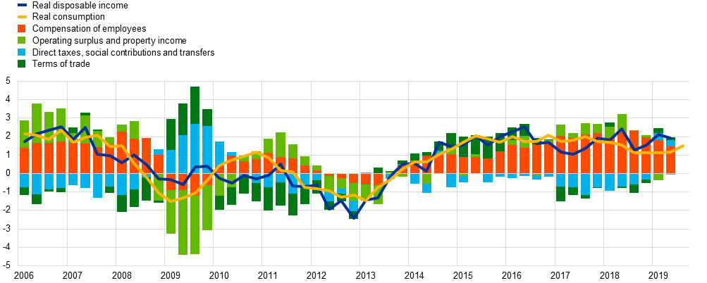
Sources: Eurostat and ECB calculations.
Notes: All income components are deflated with the GDP deflator. The contribution from the terms of trade is proxied by the differential in the GDP and consumption deflator. Consumption and total disposable income are deflated with the consumption deflator.
Latest observation: Q3 2019 for real consumption and Q2 2019 for the rest.
Euro area consumer confidence
(percentage balances, deviation from mean)
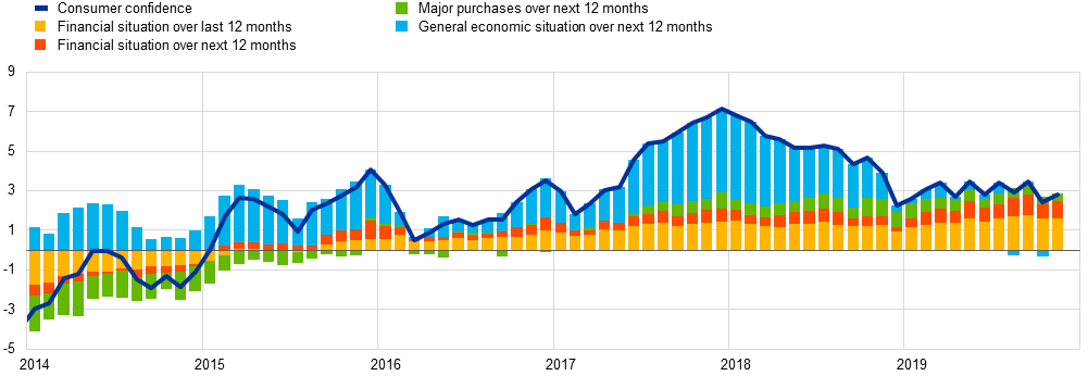
Sources: European Commission and ECB calculations.
Latest observation: November 2019.
Household investment
(year-on-year percentage changes)
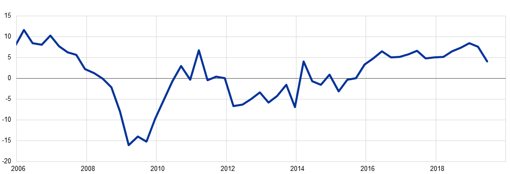
Sources: Eurostat and ECB.
Note: The data refer to nominal gross fixed capital formation by households and non-profit institutions serving households.
Latest observation: Q2 2019.
For monetary policy analysis, an important question is the extent to which easier financial conditions have contributed to these dynamics through a variety of direct and indirect channels. A comprehensive analysis of this question requires a microeconomic approach, which takes into account relevant differences across households.[2]
Household-level data, such as those available from the HFCS, are essential for this purpose. These data highlight some quantitatively-important dimensions of heterogeneity in the euro area, which can be grouped into two broad categories.
First, the level and volatility of income varies across households according to socio-economic characteristics such as education, age and occupation.[3] Households with different income sources (e.g. employees, firm owners, unemployed), different skill levels, or different labour supply elasticities will respond differently to macroeconomic shocks. In turn, wages vary strongly with characteristics such as age and education. Such differences not only matter for understanding how different types of households react differently to economic shocks: evidence suggests that changes in the composition of the workforce can help explaining euro area wage growth at the aggregate level.[4]
Estimates for the largest four euro area countries indicate that the increase in income after an expansionary monetary policy shock is particularly large for households in the lowest income quintile (Chart 4).[5] The explanation is that low-income households are substantially more likely to be unemployed at any point in time: it follows that this group is more likely to benefit from the employment creation triggered by a monetary expansion. Similarly, the elasticity of labour income in relation to changes in aggregate GDP growth is significantly higher for workers in lower-income households.[6]
Effect of monetary policy easing on household income by income quintile
(percentages)
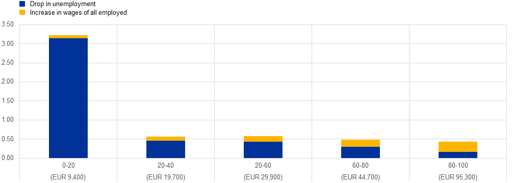
Sources: Lenza, M. and Slacalek, J. (2018) op. cit., Eurosystem Household Finance and Consumption Survey, wave 2.
Notes: The chart, taken from Lenza, M. and Slacalek, J. (2018) op. cit, shows the percentage change in mean income across income quintiles in the euro area four quarters after the impact of a quantitative easing shock, which is assumed to correspond to a 30 basis point drop in the spread between a 10-year sovereign bond and the policy rate. It also shows the decomposition of the change into the extensive margin (transition from unemployment to employment) and the intensive margin (increase in wages). The numbers in brackets show the initial levels of mean gross household income in each quintile. The statistics cover the euro area, which is modelled here as an aggregate of France, Germany, Italy, and Spain.
Second, households differ substantially in the size and composition of the assets they own and in their indebtedness (Chart 5). Based on the second wave of the HFCS almost 60 percent of euro area households are homeowners, of which about a third have a mortgage. Almost all households own financial assets, even if their value is typically only a small fraction of the value of their real estate holdings.[7] These dimensions of household heterogeneity clearly matter for the exposure of individual households to monetary policy decisions.
Household assets and debt by income quintile
(x-axis: quintiles and deciles; y-axis: EUR thousands)
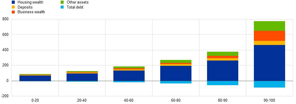
Sources: De Bond, G. et al. (op. cit), and Household Finance and Consumption Survey, results from the second wave.Notes: The chart shows the average value of assets and debt per household across five income quintiles for the euro area. The top quintile is further broken down into two deciles. Housing wealth is composed of the households’ main residence and other real estate. Other assets include the value of households’ vehicles, voluntary pension/life insurance, shares, valuables, bonds, managed accounts and money owed to households.
For instance, ECB simulations suggest that unexpectedly-low inflation tends to harm young and middle-aged households, and more so for young income-rich households that disproportionately have nominal debt liabilities. [8] By contrast, older households tend to gain from unexpectedly-low inflation, especially if they are income-rich, since this group tends to hold nominal assets.[9]
To the extent that their financial assets have short maturities and their mortgages have adjustable rates, households will also be differently affected by a reduction in the interest rate.[10] The estimates in Chart 6 show that an average net borrower has gained close to EUR 2,000 per year in lower interest payments in recent years, whereas an average net saver has lost close to EUR 700 per year.[11]
Change in net interest income for borrowers and savers in the euro area
(euros per household; change in annual net interest income, 2007-2017)
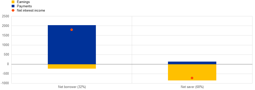
Sources: Dossche, M. et al. op. cit., using the Household Finance and Consumption Survey (second wave).
Notes: Net borrowers are defined as households with a negative net financial wealth position and net savers are defined as households with a positive net financial wealth position. Percentages in brackets indicate the share of net borrowers and net savers in the total household population.
Analogously, only homeowners will benefit from any increase in house prices induced by a monetary policy easing and those with mortgages will benefit disproportionately due to the impact of leverage. Conversely, Chart 7 reports estimates of the evolution of household net wealth as a result of the lower house prices observed in many countries between 2011 and 2014. It suggests that the net wealth of homeowners declined by 6 percentage points more than the wealth of renters. The decline was especially marked for homeowners with mortgages, for whom it amounted to as much as around 20 percent.
Growth of median net wealth by housing status, 2011-14
(HICP-adjusted; percentages)
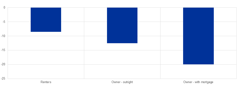
Source: Household Finance and Consumption Survey, waves 1 and 2.
Note: The chart shows the growth rates of the median net wealth in the euro area for outright owners, owners with a mortgage and renters from 2011 to 2014, deflated by the HICP.
Assessing the overall implications of these many dimensions of heterogeneity is challenging. Recent ECB research suggests that the most important dimension of heterogeneity is related to employment status.[12] Following an easing of monetary policy conditions, there are disproportionate increases in income in the lower part of the income distribution, which results in a decline in measured income inequality. By contrast, since a majority of households are homeowners, an increase in house prices due to a looser monetary policy has a relatively even impact of house prices across the wealth distribution.[13] At the same time, it is worth keeping in mind that the degree of home ownership can vary considerably across countries. The more concentrated ownership of equities and bonds among households means that this component of the wealth distribution varies with the monetary stance, even while recalling that many households have indirect financial holdings through pension funds and other types of investment vehicles.
From a broader perspective, we should also bear in mind that the contribution of monetary policy to changes in inequality is small, compared with the role of fiscal policy (especially the degree of redistribution in the design of the tax and transfer systems) and structural economic trends.
Differences across households also matter for the relation between aggregate income and aggregate consumption. In particular, if an increase in aggregate income is not uniform across households, the overall consumption response will depend on the marginal propensity to consume that is, the fraction of an additional euro received that is spent on consumption – of the different household types. A rich empirical literature has uncovered considerable heterogeneity in marginal propensity to consume across household types. In particular, this literature finds that the spending decisions of households owning few liquid assets are much more sensitive to shocks than the spending decisions of households that own sufficient liquid buffers. Similarly, highly-indebted households tend to have a higher propensity to consume than savers.[14]
Quantifying the implications for the transmission of monetary policy of heterogeneity in the marginal propensity to consume requires detailed institutional and socio-economic information on households at higher frequency. This type of information is available in certain countries and it is encouraging that researchers are starting to make use of it.[15] The results indicate that this heterogeneity does play a role in shaping the transmission of monetary policy. Beyond the intertemporal substitution channel, other channels have been highlighted by the expanding literature on heterogeneous-agent New Keynesian (HANK) models.[16] These include: a “cash-flow” channel, through which the decline in debt service for debtors means that they have more of their income available for spending; an “income” channel, whereby higher consumption expenditure results from the increase in employment and wages; and a “wealth” channel, such that the increase in asset valuations generates more spending through wealth effects.
Some initial estimates of the quantitative impact of all these channels are also available for the euro area. They are reported in Chart 8, where households are classified into three groups: (i) renters with limited financial assets; (ii) homeowners with limited financial assets but possibly a (sizable) mortgage; and (iii) homeowners with adequate financial assets. According to this classification, 10 percent of households in the euro area are renters with limited financial assets, 12 percent are homeowners with limited financial assets and 78 percent are homeowners with adequate financial assets.
Effects of a 100 basis point cut in interest rates on consumption in the euro area, depending on household wealth
(change in consumption; percentages)
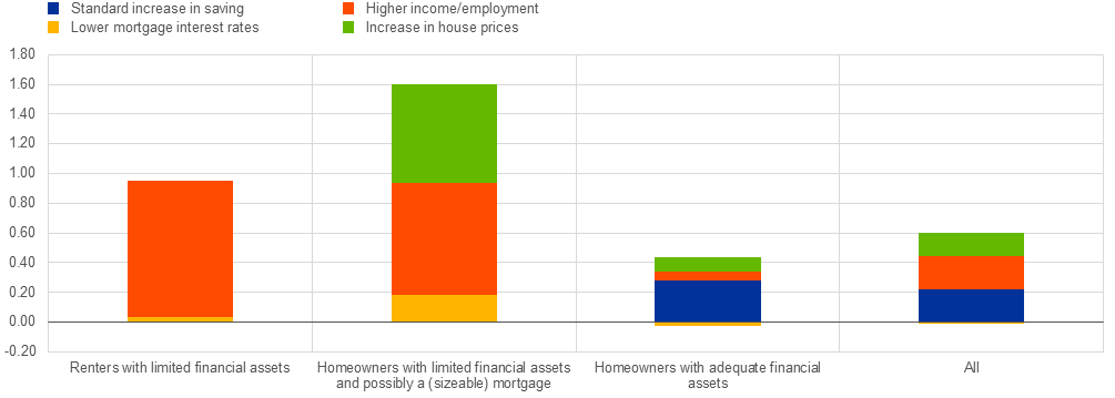
Source: Slacalek, Tristani and Violante (2019), Household Finance and Consumption Survey, wave 2.
Notes: The figure shows a decomposition of the effects of a 100 basis point cut in interest rates on consumption. The total consists of four parts. The standard intertemporal substitution effect (IES), the cash-flow effect, the income effect and the housing wealth effect. The size of these effects varies depending on households’ wealth. Euro area in this chart refers to France, Germany, Italy and Spain.
This classification is relevant, since it has been argued that the two groups of households with limited financial assets are more constrained in their ability to smooth consumption over time and tend to respond more strongly to temporary changes in income.[17] In addition, the composition of wealth of the different groups varies: while homeowners with limited financial assets tend to have a mortgage (and their debt service decreases when the policy rate is cut), the homeowners with substantial financial assets often experience lower returns on interest-rate-bearing assets if the policy rate declines.
Chart 8 decomposes the overall effect on consumer spending into the components attributable to the various transmission channels.[18] First, the standard, intertemporal substitution channel is present only for financially-unconstrained households which are able to save. It makes up only about a third of the total impact on aggregate consumption. Second, the cash-flow channel is particularly strong for homeowners with limited financial assets, who tend to have large mortgages, often with adjustable rates. Third, spending is substantially stimulated via the income channel. This channel is heavily skewed towards lower-income households, who also tend to benefit disproportionately from a stronger labour market. Fourth, the strongest asset price effect occurs through the increases in house prices. This effect turns out to be quite large for highly leveraged homeowners, since their consumption is more sensitive to house prices.[19]
Overall, the spending of the lower-income cohort and the cohort of homeowners with only limited financial assets is much more strongly stimulated by monetary policy easing. A 100 basis point cut in interest rates increases consumption of these groups by almost 1.0 percent and 1.6 percent respectively, while consumption of the financially-unconstrained group increases only by 0.4 percent.
These estimates suggest that the standard intertemporal substitution channel substantially contributes to the spending decision of many households, but the other three channels, which have traditionally been neglected, are decisive for the consumption choice of the lower-income cohort and highly-leveraged homeowners. These three channels contribute about two thirds of the total response of aggregate consumption to a monetary policy shift. It follows that household heterogeneity can help to explain how the effects of monetary policy can be relatively large, due to the larger consumption response of the hand-to-mouth group, even if the intertemporal substitution channel is weaker than in the representative agent framework.[20]
To summarise, it is important to account for heterogeneity in the transmission of monetary policy, but this is not a simple exercise. Comparisons between “winners and losers” based on a single channel, or a specific factor, are necessarily incomplete and likely to prove misleading.
Concluding remarks
Let me conclude. Attention to variation across households and its relation to monetary policy is welcome. It helps us to make progress in understanding the key features of the transmission mechanism of monetary policy.
It is also very promising that the economics profession is finding ways to incorporate relevant dimensions of household heterogeneity in our models. This flourishing field recognises that monetary transmission is more complicated and dependent on many institutional features than suggested by the traditional representative-agent model.
Further advances will require more data and more analysis. An essential source to estimate these effects in the euro area is the HFCS. One avenue is to make use of the administrative data available in other datasets (including tax data and credit registers) to complement and improve the information collected via household surveys. I very much applaud this effort. Another important element is to better understand how consumers form expectations.[21] To this end the ECB is working on establishing a Consumer Expectations Survey, which we hope will provide a useful basis to deepen our understanding of consumer behaviour at a granular level and the extent to which this matters for macroeconomic outcomes.
- [1]I am grateful to Maarten Dossche, Jirka Slacalek, and Oreste Tristani for their contributions to this speech.
- [2]For modelling approaches that just rely on aggregate data, see: Woodford, M. (2003), Interest and Prices: Foundations of a Theory of Monetary Policy, Princeton University Press, Princeton; Smets, F. and Wouters, R. (2007), “Shocks and Frictions in US Business Cycles: A Bayesian DSGE Approach”, American Economic Review, Vol. 97(3), pp. 586-606; Del Negro, M. and Schorfheide, F. (2013), “DSGE Model-Based Forecasting”, in Elliott, G., Granger, C. and Timmermann, A. (eds.), Handbook of Economic Forecasting, Vol. 2, pp. 57-140; and Christiano, L.. J., Motto, R. and Rostagno, M. (2014), “Risk Shocks,” American Economic Review, Vol. 104(1), pp. 27-65. Some limitations of macro-only analysis (such as excess sensitivity of consumption to interest rates) are highlighted by: Campbell, J. Y. and Mankiw, N. G. (1989) “Consumption, Income and Interest Rates: Reinterpreting the Time Series Evidence,” in Blanchard, O. J. and Fischer, S. (eds.), NBER Macroeconomics Annual 1989, Vol. 4, National Bureau of Economic Research, pp. 185-246; and Canzoneri, M. B., Cumby, R. E. and Diba, B. T. (2007), “Euler equations and money market interest rates: A challenge for monetary policy models,” Journal of Monetary Economics, Vol. 54(7), pp. 1863-1881. For an aggregate perspective on household wealth and consumption, see de Bondt, G., Gieseck, A. and Tujula, M. (forthcoming), “Household wealth and consumption in the euro area”, Economic Bulletin, ECB.
- [3]The implications of the demographic structure of the population for the response of different age cohorts to a monetary policy shock is considered in Leahy, J. V. and Thapar, A. (2019) “Demographic Effects on the Impact of Monetary Policy”, NBER Working Paper Series, No 26324, National Bureau of Economic Research.
- [4]See Nickel, C., Bobeica, E., Koester, G., Lis, E. and Porqueddu, M. (eds.) (2019), “Understanding low wage growth in the euro area and European countries”, Occasional Paper Series, No 232, ECB.
- [5]See Lenza, M. and Slacalek J. (2018), “How does monetary policy affect income and wealth inequality? Evidence from quantitative easing in the euro area”, Working Paper Series, No 2190, ECB.
- [6]See Dossche, M. and Hartwig, J. (2019), “Household income risk over the business cycle,” Economic Bulletin, Issue 6, ECB.
- [7]Comparing the median of the total value of financial asset holdings to the median of the total value of real estate holdings, computed across those households owning real estate.
- [8]Asymmetric effects of a monetary easing also discussed in Doepke, M., and Schneider, M. (2006), “Inflation and the Redistribution of Nominal Wealth,” Journal of Political Economy, Vol. 114, Nol 6, 1069–1097; Adam, K., and Zhu, J. (2016), “Price-Level Changes and the Redistribution of Nominal Wealth across the Euro Area,” Journal of the European Economic Association, Vol. 14, No 4, 871–906.
- [9]See Box 4.3 in Household Finance and Consumption Network (2016), “The Household Finance and Consumption Survey — results from the second wave,” Statistics Paper Series, No 18, ECB.
- [10]See Auclert, A. (2019), “Monetary Policy and the Redistribution Channel,” American Economic Review, Vol. 109(6), pp. 2333–2367; see also Tzamourani, P. (2019), The Interest Rate Exposure of Euro Area Households, Discussion Paper Series, No 01/2019, Deutsche Bundesbank.
- [11]See Dossche, M., Hartwig, J., Pierluigi, B., and Velasco, A. (2019), “The redistribution of interest income in the euro area, 2008-2018,” mimeo.
- [12]Lenza, M. and Slacalek, J. (2018), “How does monetary policy affect income and wealth inequality? Evidence from quantitative easing in the euro area”, Working Paper Series, No 2190, ECB.
- [13]Quantitatively, these results may differ across countries, depending on, for example, the reaction of employment and house prices to monetary policy. At the same time, qualitatively these results also hold across large euro area countries, see Lenza and Slacalek op. cit. for details.
- [14]See the reviews of the empirical literature by Jappelli, T. and Pistaferri, L. (2010), “The Consumption Response to Income Changes,” Annual Review of Economics, Vol. 2(1), pp. 479–506; Carroll, C. D., Slacalek, J., Tokuoka, K. and White, M. N. (2017), “The Distribution of Wealth and the Marginal Propensity to Consume,” Quantitative Economics, Vol. 8, pp. 977–1020, Table 1; and Crawley, E. S., and Kuchler A. (2018), “Consumption Heterogeneity: Micro Drivers and Macro Implications,” Working Paper, No 129, Danmarks Nationalbank, Table 1. A related paper builds on heterogeneity in marginal propensities across savers and borrowers see Mian, A., Straub, L. and Sufi, A. (2019), “Indebted Demand,” Harvard University, mimeo.
- [15]See Fagereng, A., Holm, M. B. and Natvik G. J. (2017): “MPC Heterogeneity and Household Balance Sheets,” Discussion Paper, Statistics Norway; and Crawley, E. S., and Kuchler, A., op. cit.
- [16]See Kaplan, G., Moll, B. and Violante, G. L. (2018) “Monetary Policy According to HANK”, American Economic Review, Vol. 108(3), pp.697-743. Of course, in addition to the New Keynesian framework, there is also a wider literature studying the implications of household heterogeneity for macroeconomic dynamics through a variety of mechanisms. See, among others, Huggett, M. (1996) “Wealth distribution in life-cycle economies”, Journal of Monetary Economics, Vol. 38(3), pp. 469-94; Heathcote, J., Storesletten, K. and Violante, G. L. (2009) “Quantitative Macroeconomics with Heterogeneous Households”, Annual Review of Economics, Annual Reviews, Vol. 1(2), pp. 319,354.
- [17]See, among others, Kaplan, G., Violante, G. L. and Weidner, J. (2014), “The Wealthy Hand-to-Mouth”, Brookings, Papers on Economic Activity, 45(1), 77–153, on the importance of accounting for hand-to-mouth households.
- [18]The figure is based on Slacalek, J, Tristani, O. and Violante, G. L. (2019), “Household Balance Sheet Channels of Monetary Policy: A Back of the Envelope Calculation for the Euro Area”, mimeo.
- [19]Slacalek et al. op. cit. also consider the effects on consumption via stock market wealth. In the euro area household portfolios are heavily skewed toward housing, except at the very top tail of the distribution. Correspondingly, Slacalek et al. op. cit. show that the effect of stock market wealth on consumption is limited, even for the non-hand-to-mouth households, also because their marginal propensities to consume out of stock market wealth are very small. This result holds even after the holdings of stock market wealth by the non-hand-to-mouth households in the survey are corrected for underreporting. Compared to aggregate sources, the survey covers about 70 percent of the stock market wealth at the euro area level.
- [20]Analogous additional amplification can occur via heterogeneity across firms due to differences in leverage and other factors; see, amongst others, Jeenas, P. (2018), “Firm Balance Sheet Liquidity, Monetary Policy Shocks, and Investment Dynamics,” Technical Report.and Ottonello, P., and Winberry, T. (2018), “Financial Heterogeneity and the Investment Channel of Monetary Policy,” Working Paper, No. 24221, National Bureau of Economic Research.
- [21]For a discussion of household expectations of inflation, see Cœuré, B. (2019) “Inflation expectations and the conduct of monetary policy”, Speech at the SAFE Policy Center on 11 July 2019.
Ευρωπαϊκή Κεντρική Τράπεζα
Γενική Διεύθυνση Επικοινωνίας
- Sonnemannstrasse 20
- 60314 Frankfurt am Main, Germany
- +49 69 1344 7455
- media@ecb.europa.eu
Η αναπαραγωγή επιτρέπεται εφόσον γίνεται αναφορά στην πηγή.
Εκπρόσωποι Τύπου