
The effects of changes in the composition of employment on euro area wage growth
Published as part of the ECB Economic Bulletin, Issue 8/2019.
1 Introduction
Until recently, wage growth in the euro area has been low and under-predicted. Looking at the period 2013-17, this weakness can be explained to a large extent by the factors traditionally captured in a Phillips curve analysis, such as economic slack and inflation expectations. Slack in the labour market can be measured by a broad range of different indicators, which include “narrow” indicators (e.g. the unemployment rate) or more unconventional measures such as the broad unemployment rate. The latter also includes euro area working age population marginally attached to the labour force – i.e. those members of the labour force categorised as inactive but still competing, albeit less actively, in the labour market.[1] In general it seems that broader measures of labour underutilisation brought some marginal gains in explaining the subdued wage growth observed in the euro area over the period 2013-17.[2] However, the factors traditionally included in a Phillips curve analysis do not paint the full picture.[3]
Could changes in the composition of employment also have contributed to low wage growth in the euro area? Wages differ, for example, across sectors and are affected by employees’ personal characteristics and contract types. These “compositional effects” can mean that changes in the composition of employment can affect average wage growth in an economy. They also depend on the degree to which the composition of employment changes and on the size of differences in wages.
In the euro area, significant changes in the composition of employment have taken place since the beginning of the crisis. These include shifts in age and level of education, as well as in the prevalence of different contract types reflecting temporary and permanent employment.[4] The sectoral composition of employment has also changed because of shifts in employees working in higher and lower-paying sectors of the economy.
Shifts in the composition of employment can be driven by trend and cyclical developments. One case in point is the age structure of employees: this can be affected by trend developments, such as an ageing population, but also by cyclical developments, such as younger workers being at a higher risk of losing their job in a downturn.
Based on the economic literature, compositional effects can have a substantial impact on wage growth. Early studies have shown that the impact of changes on the composition of employment can be sizeable,[5] and the results of more recent studies focusing on the period of the crisis are similar.[6]
Can such compositional effects help us understand the development of wage growth over the cycle? They can do, for example, if compositional effects are heavily influenced by the cycle, pushing up wage growth in a downturn or depressing wage growth in an upturn. According to the literature, compositional changes in employment may indeed lead to such a countercyclical effect on aggregate wages.[7]
This article assesses how compositional effects have affected wage growth in the euro area and its member countries since 2007.[8] For our analysis we mainly rely on microdata from the EU Survey on Income and Living Conditions (EU-SILC). The article also includes cross-checks based on the EU Labour Force Survey (EU-LFS) and national accounts data. After a discussion of some conceptual foundations, we introduce the data used and illustrate recent changes in employment composition in the euro area. This is followed by an outline of our approach to assessing compositional effects and, finally, a discussion of evidence of the role of compositional effects for the euro area as a whole and the contribution of individual euro area countries.[9]
This article finds that compositional effects have contributed to a subdued reaction of wages in the euro area over the business cycle – including in the period of low wage growth. Compositional effects pushed up wage growth early in the crisis, but have since decreased and turned negative. This has contributed to a relatively muted response from aggregate wage growth, both to the strong downturn of the labour market early in the crisis and later to cyclical improvements during the years after 2013. The most important contributions to compositional effects seem to have been related to changes in the age and educational structure of employment, which have had both a long-term and a cyclical impact. The countercyclical pattern of compositional effects resulted mainly from the group of young and comparatively low-skilled workers with relatively low wages; this group was hit especially hard by job losses early in the crisis (pushing average wage growth up during the downturn) and only experienced higher re-employment probability during the recovery period (with a downward effect on average wage growth). Looking at country-specific evidence, the euro area aggregate results have been influenced by Spain and Italy in particular.
Conceptually, it would be appealing to estimate a Phillips curve for wage growth net of compositional effects, but this seems to be very difficult to implement. With respect to data availability, such an approach is complicated by (i) the annual frequency of data needed to calculate compositional effects, (ii) the short length of the time series, and (iii) the substantial time lags in publication of the data.[10]
2 The effects of changes in the composition of employment on wage growth – conceptual foundations
Differences in wages can be observed in various dimensions and can vary based on workers’ individual characteristics and across sectors. As labour productivity differs strongly across sectors, wages vary. They tend, for example, to be higher in the industrial sector of the economy than in the services sector. Another factor accounting for differences in pay is level of education, with higher levels of education being correlated with higher skills and thus higher wages. Contract type may also play a role, depending on whether individuals work part-time or full-time, and whether they are employed on a temporary or permanent basis.[11]
Based on differences in wages across individuals and sectors, changes in the composition of employment can affect both the average level and the growth rate of wages in an economy. Key indicators for wages in an economy are compensation per employee (CPE) or compensation per hour (CPH). CPE is the sum total of employees’ compensation divided by the total number of employees, and CPH is the sum total of employees’ compensation divided by the total number of hours worked in the economy. Employees’ compensation includes not only wages and salaries in cash but also wages and salaries in kind, as well as employers' social contributions. Sectoral shifts in employment composition in the industrial sector, with its relatively high wages, can, for example, cause CPE and CPH to increase. In a similar vein, an increasing share of employees with high levels of education can also have a positive effect on average CPE and average CPH in an economy.
Changes in the composition of employment can have implications for wage growth based not only on differences in wage levels but also on differences in wage growth among different types of workers. One example is older workers tending to have higher wage levels but experiencing slower wage growth than younger workers. While both effects need to be taken into account, the effects resulting from the difference in wage levels, at least in the short run, seem to be dominating.[12]
While compositional effects based on sectoral developments can, to a certain extent, be analysed based on macrodata from national accounts, studying the impact of individual employees’ characteristics requires the use of microdata. The effects of sectoral shifts in employment can, to a certain level of sectoral granularity, be analysed based on national accounts data for employment and compensation. However, comprehensive and consistent datasets for the euro area, including data on employment composition based on individual employees’ characteristics and their wages, are only available based on surveys (see Box 2 for a discussion of available data).
Drivers of compositional effects may be of a cyclical or structural nature. Structural developments, such as ageing, are likely to have a slow-moving compositional effect on wage growth, since older employees tend to have higher wages.
Cyclical developments drive compositional effects, especially due to differences in the risk of losing or gaining employment. Employment risk over the business cycle is unequally distributed with respect to workers’ skills and characteristics. During downturns and upturns, job losses and gains have the greatest effect on lower-skilled and younger workers. This is supported by research both in the United States and Europe.[13]
Compositional effects can be countercyclical and may contribute to a muted reaction from wage growth to the business cycle. If lower-skilled and younger workers, who are more likely to receive relatively low wages, are particularly likely to lose their jobs in a downturn, average wage growth (measured by CPE and CPH, for example) is pushed up mechanically. On the other hand, the reintegration of these workers into employment in an upturn depresses average wage growth. Such countercyclical compositional effects can partially mute the “true” cyclical reaction of wages to changes in the labour market.
Empirical studies have indeed found a countercyclical pattern of compositional effects in the euro area and some EU countries.[14] Such countercyclical effects have been found in empirical studies of the euro area in the early part of the crisis[15] and also in country-specific studies for Belgium[16], Italy[17] and the United Kingdom[18].
Trend developments might have a pronounced impact on compositional effects but are unlikely to cancel out possible cyclical patterns. Overall, compositional effects are likely to reflect both trend and cyclical developments, the roles of which can vary over time depending on how pronounced a trend or cyclical development is. However, even if trend developments are very pronounced, they are unlikely to cancel out possible countercyclical patterns. This is because structural changes are usually uncorrelated with the business cycle.
Box 1 Effects of changes in the sectoral composition of employment on wage growth
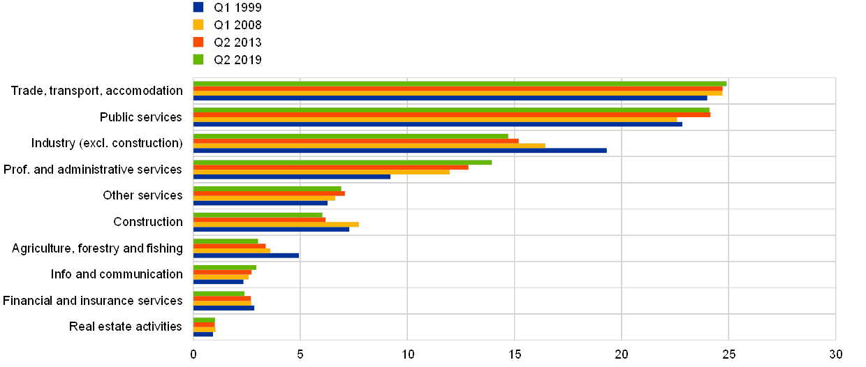
As wage levels differ across sectors in the economy, changes in the sectoral composition of employment can affect aggregate wage growth.[19] These differences are often linked to variations in labour productivity. The size of the effects on aggregate wage growth depends both on the extent of sectoral shifts in employment and on the size of differences in pay. For example, a rise in the share of employment in sectors with low wage levels can dampen wage growth. These sectoral changes can be analysed on the basis of national accounts data, which are available for ten main sectors (see Chart A).
Sectoral shifts are driven both by trend and cyclical developments. For example, a long-term reallocation of employment from industry to market and public services is observable (see Chart A). This longer-term trend is in line with developments in terms of value added, but may also be related to increasing automation in industry and the limited scope for that in the services sector. In the public sector, one main structural driver of increased employment is likely to be the demand for healthcare, which is related to the ageing of a society (among other things). The business cycle also has an impact on the sectoral composition of employment. This is most clearly visible in the concentration of the labour market adjustment during the crisis, primarily in the industrial and construction sectors.
Chart A
The composition of euro area employment by sector
(share of sectors in total employment, percentages)
Source: Eurostat.
The sectoral composition of employment growth in the euro area over the recovery period would suggest a downward impact on overall wage growth. Since the second quarter of 2013 – the start of the economic and labour market recovery – employment has grown most strongly in the services sectors. Wage levels in these sectors – such as in professional and administrative services, or trade transport and accommodation – are close to or below euro area averages (see Chart B). At the same time, employment growth was relatively small or negative in some sectors characterised by high wage levels, including financial and insurance services, information and communication services, and industry (excluding construction).
Chart B
Changes in euro area employment by sector and sectoral wage levels over the recovery period
(x-axis: change in employment; y-axis: average quarterly compensation in euro)
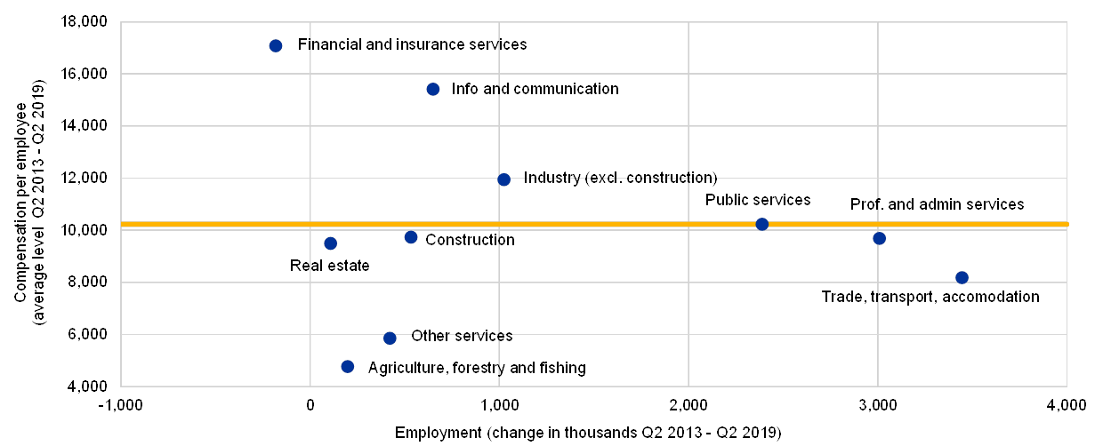
Source: Eurostat.
However, shifts in sectoral composition seem to have had only a very limited effect on aggregate wage growth in the euro area overall. Effects of changes in the sectoral composition on wage growth can be identified by comparing realised aggregate wage growth with a counterfactual series for wage growth, which keeps sectoral shares in overall employment constant. Fixing sectoral weights at their 2008 level reveals that such sectoral shifts have most likely had only a very limited effect on overall wage growth (see Chart C).
Chart C
Growth of compensation per employee with changing and fixed sectoral weights
(annual percentage changes)
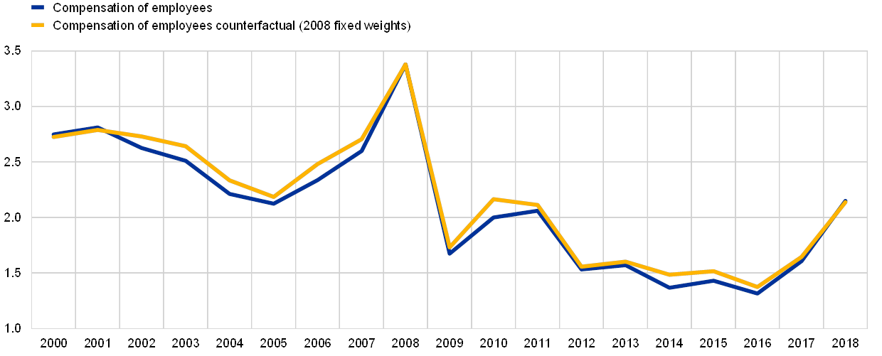
Sources: Eurostat and ECB calculations.
This box finds that shifts in the sectoral composition of employment do not seem to have had a major influence on wage growth. This could also be seen as an indication that microdata studies, like the one pursued in the main text, can also shed some light on within-sector shifts.[20]
3 Developments in the composition of employment and wage differences across employee characteristics
In the euro area, significant changes have taken place in the age and educational structure of employment (see Chart 1).[21] This can be illustrated based on microdata from EU-SILC, which are available up to and including 2016[22] (see Box 2 for details and a comparison of EU-SILC data with alternative available datasets; see Box 4 for a cross-check against data from the EU-LFS). Most importantly, the share of older employees has increased, while the share of younger workers has decreased substantially. At the same time, the share of employees with a lower level of education has decreased, while the share of more highly educated employees has increased.
Chart 1
Development of the main characteristics related to employment in the euro area according to the EU-SILC
(percentages)
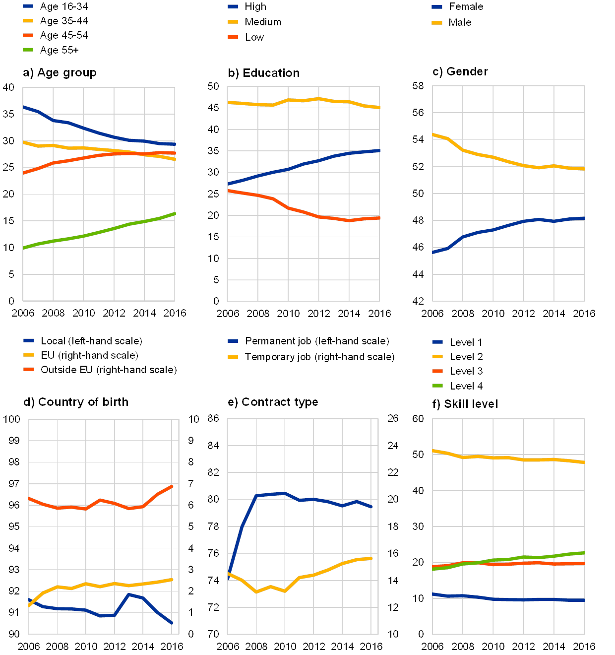
Sources: Eurostat (EU-SILC) and ECB staff calculations.
Notes: Euro area aggregate weighted by hours worked; numbers not adding up to 100% indicate missing data. The skill levels are defined by grouping different occupational groups: level 1 includes elementary occupations; level 2 includes clerical support workers, service and sales workers, skilled agricultural, forestry and fishery workers, craft and related trades workers, and plant and machine operators and assemblers; level 3 includes technicians and associate professionals; and level 4 includes managers and professionals.
These developments can be partly attributed to longer-term trends (demographic changes, pension system reforms, the trend towards higher levels of education, etc.) but can be also related to cyclical developments in some countries: younger and less educated/skilled workers were the first to lose their jobs during the crisis, further increasing the share of older and more highly educated employees. This cyclical pattern is also observed in the development of temporary contracts, the number of which declined early in the crisis in a number of countries but whose share increased during the recovery.
Chart 2
Mean income per group of employees compared with overall mean income
(euro area, 1 = mean income)
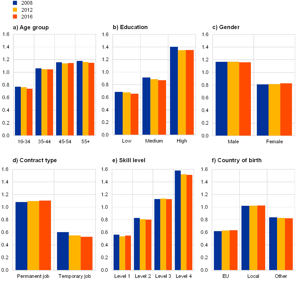
Sources: Eurostat (EU-SILC) and ECB staff calculations.
Notes: Weighted by hours worked. The skill levels are defined by grouping different occupational groups: level 1 includes elementary occupations; level 2 includes clerical support workers, service and sales workers, skilled agricultural, forestry and fishery workers, craft and related trades workers, and plant and machine operators and assemblers; level 3 includes technicians and associate professionals; and level 4 includes managers and professionals. The income variable used is wage per hour as derived from EU-SILC variables.
The developments in the composition of employment, together with considerable differences in the mean income of the different groups, motivates the assessment of compositional effects on wage growth. A comparison of the euro area mean income of different age groups with the mean income of all employees (see Chart 2) shows that workers over the age of 44, in particular, earn considerably more than workers between the ages of 16 and 34, the wages of the latter being, on average, less than 80% of the overall mean. The difference is even more notable when comparing employees across different levels of education: while less highly educated employees earn around 60% of the mean, more highly educated employees earn between 20% and 40% more than the mean (depending on the year). Similar differences can be observed when comparing employees’ occupations, skill levels, genders, contract types and nationalities.
Box 2 Available microdata for studying compositional effects in euro area wage growth
Microdata that include characteristics of individual workers and cover EU or euro area countries in a consistent way are only available on the basis of surveys. Administrative data based on social security systems, for example, are only available in some countries,[23] which does not allow for a consistent approach covering all euro area countries.
The main survey-based microdata that can be used to describe the labour market and income statistics in EU countries are the Statistics on Income and Living Conditions (EU-SILC), the EU Labour Force Survey (EU-LFS) and the Structure of Earnings Survey (SES). Their main features are depicted in Table A. Contrary to macro-level data, e.g. from national accounts, which provide aggregate information, these datasets include micro-level data at the individual and/or household level.
Table A
Main features of different sets of microdata describing the labour market

The analysis presented in this article is based on the EU-SILC dataset, which is “the reference source for comparative statistics on income distribution and social inclusion in the European Union”[24]. It is an annual survey conducted in all EU and some non-EU countries.[25] The data are collected by National Statistical Institutes and disseminated by Eurostat. The survey offers a wide range of variables related to individual, job-related and firm-related characteristics as depicted in Table B. For the analysis in this article, the cross-sectional dataset[26] is used, which is currently available for the survey years from 2005 to 2017[27].
Table B
Selected variables included in the different sets of microdata, including variables with potential relevance for compositional effects
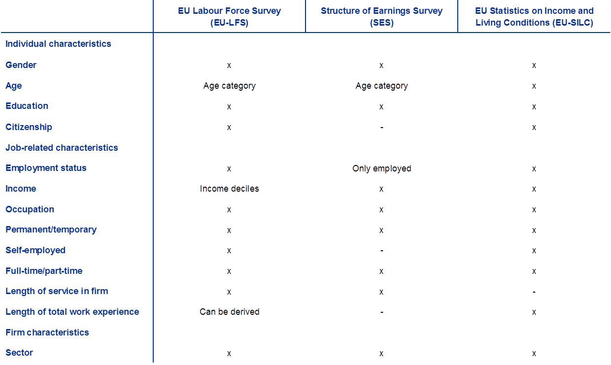
Compared with EU-LFS and SES data, the EU-SILC data offer a range of advantages for an analysis of the contribution of compositional changes in the labour force to wage growth. Most importantly, the EU-LFS only provides information on income in the form of income deciles for a country as a whole, which does not allow for an analysis of the effects of individual characteristics on wages.[28] Still, it is a valuable data source that – unlike the EU-SILC – offers very timely statistics on labour market developments (see also Box 4). The SES, on the other hand, includes rich and detailed information on the relationship between wages and workers’ individual characteristics, but is only conducted once every four years. This prevents analyses of changes in compositional effects from year to year. Furthermore, the survey includes individuals in firms with at least ten employees for most countries (see Table A), and thus excludes an important share of individuals who would ideally be included in an analysis of compositional effects.
Trends in aggregate hourly wage growth as calculated from the EU-SILC are broadly consistent with wage growth from national accounts. In some cases, however, differences exist.[29] Mismatches may relate to differences between the survey target population and national accounts, and small differences in variable definitions (e.g. hourly wages). For example, the survey might not fully capture special (i.e. temporary) working time adjustments or short-term changes. Furthermore, the EU-SILC target population is the resident population in private households of the survey country but excludes cross-border workers and “collective households”, e.g. immigrants in temporary housing arrangements.
4 Evidence of compositional effects in the euro area
4.1 Microdata evidence for compositional effects based on individual characteristics of the euro area
Analysing the effects of changes in the composition of employment on aggregate wage growth requires the effects from changes in the characteristics of employment to be disentangled from the changes in the individual returns. Disentanglement can be achieved using the “Oaxaca-Blinder decomposition” technique, which is the general approach we have taken for our analysis.
The compositional effect calculated using the Oaxaca-Blinder decomposition measures the mechanical differences in aggregate wages due only to the changed composition of employees. Box 3 describes the methodology in greater detail.
The dependent variable in our analysis is hourly gross wage growth, while the independent variables in a “baseline” configuration include the individual characteristics of age, education, gender and nationality.[30] Owing to the nature of the survey, the data represent annual averages. We weight all results with hours worked[31] during the decomposition.[32]
Sectoral and firms’ characteristics are not included in the analysis, as they are part of the market structure and would lead to an “artificial” inflation of the compositional effect. There are several arguments against including these characteristics: first, sectoral and firm characteristics may be correlated with individual characteristics, decreasing the impact of the individual characteristics. Furthermore, adding a covariate correlated to wages will increase the overall estimated composition effect, leading to overestimation.[33] Finally, as shown in Box 1, changes in sectoral composition do not seem to have had a decisive influence on wage growth in the euro area.
Box 3 Estimating compositional effects on euro area wage growth based on microdata from the EU Statistics on Income and Living Conditions (EU-SILC)
The Oaxaca-Blinder[34] decomposition is the standard approach used to study the effects of compositional changes on labour market outcomes. The method has been used in studies covering a wide array of topics, from inequality to discrimination and demographics, in order to explain the change in the means of an outcome variable between groups. This gap is decomposed into the part that is due to changes in the determinants of an outcome and the part that is due to changes in the effects of these determinants. In our case the outcome variable is the wage, and the determinants are worker skills and characteristics. The Oaxaca-Blinder decomposition of aggregate wage growth disentangles effects owing to a change in the weighting of groups (composition change), a change in individual returns (returns effect) and a simultaneous change of both (interaction term).
The estimation of compositional effects requires the availability of individual-level data containing wages and skill characteristics. In order to determine, for example, whether an increase in the average wage is due to a nominal increase in returns to skills or to a change in the skill distribution of employment, an accurate estimate of the returns to skills for each year is required. As shown in Chart A, if both the average skills (S) and the returns to skills (R) change at the same time (right-hand figure), the observed wage growth ( ) may be understated. Thus, to accurately estimate the impact of the composition changes we first need to determine the returns to skills using individual-level wages and characteristics.
Chart A
Decomposing wage growth into returns growth and average skill level
Aggregate wages and skills over two consecutive years
(average wage, average skill level)

Note: Authors’ illustration.
The Oaxaca-Blinder decomposition uses a series of regressions to disentangle compositional effects from changes in individual returns. First, the two different years are defined as two groups of employed individuals (group and group ), the individual wage (Y) and workers’ characteristics (X). The difference of the mean wage can be written:
Given a linear model:
it can be proven that:
The first term on the right-hand side of equation (3) is the compositional effect, measuring the differences in predicted wages due only to changes in the composition of the employed workforce. The second term is the coefficient effect, which measures the difference in wages (or the returns to the covariates) if the skillset of the workers is kept constant. The last term is the interaction effect, which accounts for the fact that differences in skills and returns coexist.
The interaction term captures changes in wages resulting indirectly from a change in the composition of the workforce. An example would be low-skilled immigration lowering the average wage of domestic workers (as a result of an increase in labour supply in this segment). In this article we exclude this term, as it goes beyond the direct (mechanical) effects of changes in the composition of employment on wage growth and could also capture effects other than those related to changes in the composition of employment. This is because shocks that are happening at the same time as the change in composition might, to some extent, be captured by the interaction term. For example, if a technology shock only hits low wage earners (i.e. the specific group that experiences the compositional change in a way different from the other groups) then the effects will be captured by the interaction term. Furthermore, this term is usually small[35] and would change the results only marginally. Nevertheless, we choose not to include it in the compositional effect, as it also captures an endogenous change in market conditions due to the composition change.
4.2 Evidence for the euro area
Euro area aggregate[36] results suggest that compositional effects pushed up wage growth early in the crisis, but the effect has since decreased and turned negative, thereby contributing to a relatively muted response from aggregate wage growth to cyclical improvements (see Chart 3). According to the results from the “baseline” configuration (see panel a in Chart 3), the largest positive contribution of compositional effects can be observed between 2008 and 2012, with compositional effects contributing more than 1 percentage point, up to about 1.5 percentage points, to wage growth.[37] The effect has been declining steadily since then, turning negative in 2015 and 2016.
The largest contribution to the overall effect comes from changes in the composition of the age and education structure. This is consistent with aggregate changes in the composition of employment, as discussed in Section 3, with the changes in age and education structure being dominant.
The declining and eventually negative impact of compositional effects is consistent with compositional effects having contributed to subdued wage growth in the euro area in recent years. Hence compositional effects could have contributed to the subdued reaction of wage growth to cyclical changes in the labour market – with compositional effects pushing up wage growth early in the crisis and the strong recovery of the labour market from 2013 onwards dampening this growth.
Different specifications are used as robustness checks – including workers’ skills – and different proxies for tenure as independent variables. As a first cross-check, education is replaced by skill level based on the employee’s occupation (see panel c in Chart 3). This is useful in cases where a large proportion of employees work in occupations not commensurate with their level of education. The second cross-check assesses the impact of adding proxy variables for tenure, including whether the individual has a permanent or temporary contract and whether the individual has changed jobs in the past year (see panels b and d in Chart 3). They are added on top of the baseline configuration. However, it is important to note that these proxies can only partially capture the concept of “tenure”, i.e. length of service with the same employer.
Chart 3
Euro area average compositional effects on wage growth
Results obtained with four different specifications
(percentage points)

Sources: Eurostat (EU–SILC) and ECB calculations.
Note: EU aggregates weighted by hours worked.
When replacing education with occupation as a proxy for skill level, the overall effect becomes more volatile and shows a less pronounced pattern for many countries. This indicates that the use of occupation as a proxy for skill level in the EU-SILC seems to be meaningful only to a limited extent. This can partly be attributed to data issues. Nevertheless, the results are in line with the overall pattern of the sign and amplitude of the compositional effects.
Adding variables that represent tenure has resulted in more negative compositional effects in recent years. The effect is illustrated in the figures in panels b and d in Chart 3, and might be explained by new hires (potentially on temporary contracts) on lower salaries coming into employment after the crisis.
Several additional checks were done but did not result in substantial changes to the results. We tested replacing “citizenship” with “country of birth”, as this seemed to be a better proxy for immigration. However, as changes in citizenship and country of birth in the EU-SILC largely follow the same trends, this did not impact the results either at the euro area aggregate level or for selected test countries.[38]
4.3 Microdata evidence for individual euro area countries
On a country-by-country basis, our analyses show a general trend in compositional effects that is similar to that for the euro area as a whole, but with some heterogeneity between countries concerning the sign and size of the effects in individual years (see Chart 4). In the configuration including proxy variables for tenure, compositional effects were positive in all countries in 2008 (see green shading in Chart 4), with effects decreasing between 2009 and 2013. This is in line with the findings for the euro area aggregate, which showed that, at the beginning of the crisis, compositional effects pushed up wage growth before later declining. For a large number of countries the results switched sign in 2014 and 2015 (see red shading in Chart 4). Large compositional effects were seen for some southern European countries in particular (e.g. Spain, Portugal and Italy), but the effect also decreased or even became negative in these countries in 2015 and 2016. Again, this sign switching is reflected in the euro area aggregate data and is driven to a significant extent by compositional changes in age and education.
Spain and Italy seem to be the main contributors to the euro area aggregate compositional effect (see Chart 5). The contribution from Spain was particularly large in 2008 but then declined, while Italy’s contribution was relatively large in 2012. In 2015 and 2016 Italy and Spain experienced very negative compositional effects; this can be explained by their respective increases in employment, which were concentrated at the lower end of the wage distribution. These results illustrate that compositional effects seem to be driven mostly by effects in countries that have experienced the largest cyclical changes in employment.[39] In line with these results, Germany and France seem to have experienced less marked compositional effects (with regard to total employment) throughout the cycle.
Chart 4
Euro area average wage growth attributed to composition changes
Results obtained for the configuration including age, education, gender, nationality and proxies for tenure
(percentage points, numbers in boxes refer to euro area weighted mean)
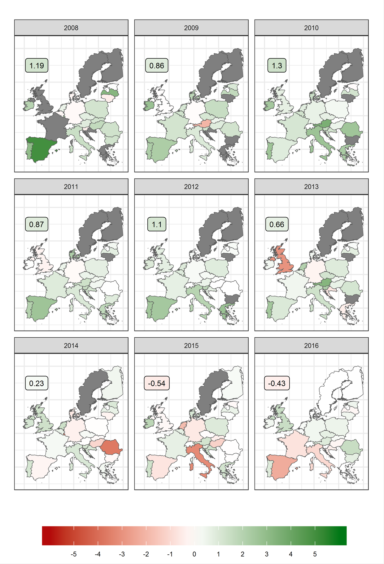
Sources: Eurostat (EU-SILC) and ECB calculations.
Notes: EU aggregates weighted by hours worked. Grey shading indicates missing data.
Negative compositional effects in recent years are mainly due to education and the reduced effect of age. Particularly in Spain and Italy – the two countries mainly driving the negative compositional effect – education has the greatest impact, as there is a stronger increase in employment among employees with a lower level of education. Furthermore, the impact of the age profile has become negative for both countries in the last two years, having previously had a strong positive effect.
Chart 5
Country contributions to the euro area compositional effect on wage growth
(percentage points)
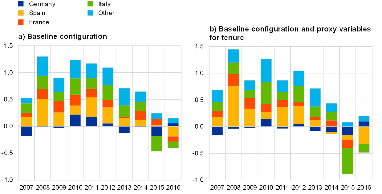
Note: ECB calculations.
Our results are consistent with studies on individual countries, such as Italy and Spain. This analysis shows significant and positive compositional effects in Italy[40] and Spain[41] during the period 2008-13.[42]
Box 4 Changes in the composition of the workforce based on the EU Labour Force Survey (EU–LFS)
This box cross-checks the extent to which the findings on compositional changes in employment derived from the EU-SILC dataset are consistent with data derived from the EU-LFS. On top of this robustness check, the EU-LFS data – which, contrary to the EU-SILC data, are already available for 2017 and 2018 – also allow a discussion on more recent developments in the composition of employment and a preliminary assessment of their possible knock-on effects on wage growth in 2017 and 2018.
The EU-LFS is a set of microdata providing detailed information on the composition of employment using several characteristics (see Box 2). It is a household survey that is conducted in all euro area countries in a harmonised way. A representative sample of individuals is regularly asked about their labour market status, personal characteristics and the characteristics of their employment (for those who are employed). This dataset is regularly used to monitor the composition of employment growth in the euro area but does not provide information on wages in a harmonised way.[43] Given that the EU-LFS is representative of the labour force, a comparison of the composition of employment in this dataset with the EU-SILC is an important robustness check for the results shown in the article.[44]
As with the developments indicated by EU-SILC data, EU-LFS data point to sizeable changes in the composition of the workforce in the euro area. The most striking change can be seen in terms of the age composition of employment. Driven by demographic developments and a significant rise in the labour force participation rate, older workers (i.e. those older than 55) account for an increasing share of employment. This age group’s share in the stock of employment in the euro area has increased from around 12% to 20% since 2006.[45] At the same time, the employment share of the more highly skilled has also increased considerably, by about 10 percentage points, while the share of those who are lower skilled has declined. The composition of employment by gender has become closer to equal, as the labour supply of women has risen considerably; however, most of this change happened before 2013. The EU-LFS also points to an increase in the share of workers with citizenship of non-euro area EU Member States. According to the characteristics of the contracts and the tasks performed, there has been a moderate shift towards temporary positions in the years to 2018, and towards occupations requiring higher skill levels.
Overall the trends in the development of workers’ individual characteristics, as found by the EU-LFS, confirm the picture given by the EU-SILC data. The two datasets provide very similar pictures, both in the composition of employment according to individual characteristics and in terms of the changes to the time period for which both are available (see Chart A). For example, although the EU-LFS points to a slightly higher share of workers with a high level of education than is reflected by the EU-SILC, the change of this share over time is very similar in the two. Remaining differences between the two datasets might be attributable to differences in the definition of variables, differences in the samples and sampling methods, and other data issues such as missing data.[46]
Chart A
Composition of employment by workers’ characteristics according to the EU-LFS and the EU-SILC
(EU-SILC = solid line, EU-LFS = dotted line)
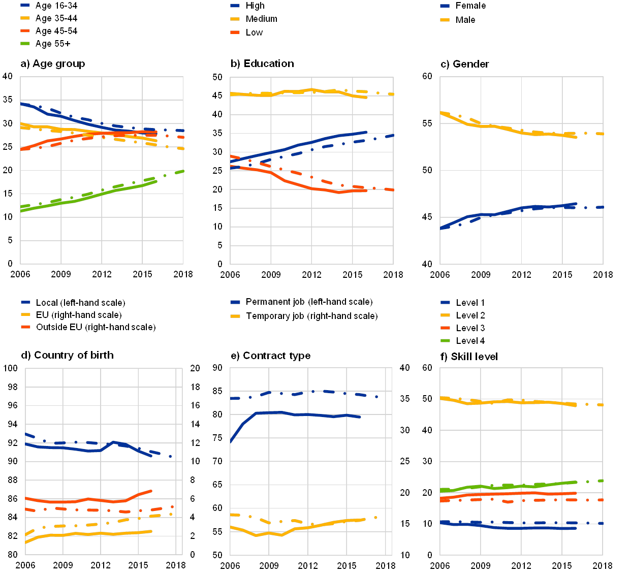
Sources: Eurostat (EU-SILC and EU-LFS) and ECB staff calculations.
Notes: Euro area aggregate weighted by hours worked; numbers not adding up to 100% indicate missing data. The decomposition according to contract type (permanent or temporary) refers to employees, while the other decompositions apply to total employment (covering employees, those who are self-employed and contributing family members). The first category, according to ages, covers people aged 15 to 34 in the EU-LFS and 16 to 34 in the EU-SILC.
More recent data from the EU-LFS indicate that some of the changes in the composition of employment have continued since 2016, for which EU-SILC data are not yet available (see Chart A). For example, the share of older workers has continued to increase and the share of workers with lower levels of education and skill has continued to decrease. These were found to be the main drivers of compositional changes in terms of aggregate wage dynamics according to the microdata analysis used in this article. Thus, the continuation of these trends suggests that we may still find some compositional effects in wage dynamics from more recent years. However, in some respects (in terms of gender, for example) the composition of employment has not changed considerably in recent years. Overall, the more limited changes in the composition of employment – especially when compared with the early years of the crisis – seem to indicate that compositional effects on wage growth might have been relatively limited in 2017 and 2018 and are unlikely to have been a major driving force behind the relatively strong recovery of wage growth in the euro area in that period. However, this can only be seen as preliminary evidence that must be reassessed once the EU-SILC data has become available for 2017 and 2018.
5 Conclusion
In the euro area, sizeable changes in the composition of employment have taken place since 2007. The share of older and more highly educated employees has increased, while the share of younger workers and those with a lower level of education has decreased. These developments can partly be attributed to longer-term trends (e.g. demographic changes, pension system reforms and the trend towards higher levels of education), but they can also be related to cyclical developments in some countries: younger and less educated/skilled workers were the first to lose their jobs during the crisis, further increasing the share of older and more highly educated employees. These patterns are confirmed by both EU-SILC and EU-LFS data.
These changes in the composition of employment seem to have pushed up wages during the crisis and contributed to subdued wage growth in recent years. An Oaxaca-Blinder decomposition applied to EU-SILC microdata suggests that these compositional effects were strongest between 2008 and 2012, but turned negative in 2015 and 2016.
A country-by-country consideration of the compositional effects shows a general trend that is similar to the trend for the euro area as a whole but with some heterogeneity among countries concerning the size of the effects in individual years. Spain and Italy seem to be the main contributors to the euro area aggregate compositional effect, while contributions from Germany and France are small with regard to total employment.
Overall, the results are robust across different specifications applied in the decomposition, and the changes in the composition of employment are also reflected in different sets of microdata. This indicates that the main developments in euro area compositional effects seem to be represented well, overall, by the analyses presented in this article.
- See, for example, the box entitled “Assessing labour market slack”, Economic Bulletin, Issue 3, ECB, Frankfurt am Main, 2017.
- See, for example, Lane, P.R. et al., “The Phillips Curve at the ECB”, speech given at the 50th Anniversary Conference of the Money, Macro & Finance Research Group, London School of Economics, 4 September 2019; Cœuré, B., “Scars or scratches? Hysteresis in the euro area”, speech given at the International Center for Monetary and Banking Studies, Geneva, 19 May 2017; and Section 2.2. of Nickel, C., Bobeica, E., Koester, G., Lis, E. and Porqueddu, M. (eds.), “Understanding low wage growth in the euro area and European countries”, Occasional Paper Series, No 232, ECB, Frankfurt am Main, September 2019.
- For the results of an ESCB Wage Expert Group, see Nickel, C., Bobeica, E., Koester, G., Lis, E. and Porqueddu, M. (eds.), op. cit.
- For details, see the box entitled “Compositional changes behind the growth in euro area employment during the recovery”, Economic Bulletin, Issue 8, ECB, Frankfurt am Main, 2018, and the article entitled “Labour supply and employment growth”, Economic Bulletin, Issue 1, ECB, Frankfurt am Main, 2018.
- See, for example, Coleman, T., “Essays on Aggregate Labor Market Business Cycle Fluctuations”, PhD Thesis, University of Chicago, 1984, Barsky, R. and Solon, G., “Real Wages over the Business Cycle”, Working Paper Series, NBER, 1988, Blank, R.M., “Why are Wages Cyclical in the 1970s”, Journal of Labor Economics, 8(1):17-47, 1990, and Kydland, F.E. and Prescott, E.C., “Cyclical Movements of the Labor Input and its Implicit Real Wage”, Economic Review, (second quarter):12-23, 1993.
- For later studies, see the box entitled “Real wages and employment composition effects during the crisis”, “Euro area labour markets and the crisis”, Occasional Paper Series, No 138, ECB, Frankfurt am Main, October 2012, and the box entitled “Real wage cyclicality in the euro area: disentangling composition from wage structure effects” in “Comparisons and contrasts of the impact of the crisis on euro area labour markets”, Occasional Paper Series, No 159, ECB, Frankfurt am Main, February 2015.
- For more details on aggregation and selection bias, see, for example, Stockman, A.C., “Aggregation Bias and the Cyclical Behavior of Real Wages”, unpublished manuscript, 1983, and Keane, M., Moffitt, R., and Runkle, D., “Real Wages over the Business Cycle : Estimating the Impact of Heterogeneity with Micro Data”, Journal of Political Economy, 96(6):1232–1266, 1988.
- The starting point of the analysis has been chosen in line with data availability and quality – see also the discussion in Box 2.
- The article builds on extensive analyses of compositional effects pursued in the context of an ESCB Wage Expert Group – see Section 3.1 of Nickel, C., Bobeica, E., Koester, G., Lis, E. and Porqueddu, M. (eds.), op. cit.
- Additionally, parts of compositional effects are likely to affect average labour productivity developments, are partially captured in Phillips curve analysis by including a productivity parameter.
- For studies on contract type and wages, see Blanchard, O. and Landier, A., "The perverse effect of partial labour market reform: fixed-term contracts in France", Economic Journal, 112, 214-244, 2002, and Booth, A.L., Francesconi, M. and Frank, J., “Temporary jobs: stepping stones or dead ends”, Economic Journal, 112(480), 2002. For more details on Germany, see Hagen, T. “Do temporary workers receive risk premiums? Assessing the wage effects of fixed-term contracts in West Germany by a matching estimator compared with parametric approaches”, Labour, 16(4), 667-705, 2002. For more details on contract type as a proxy for tenure, see Carneiro, A., Guimarães, P. and Portugal, P., “Real Wages and the Business Cycle: Accounting for Worker, Firm, and Job Title Heterogeneity”, American Economic Journal: Macroeconomics, 4(2):133–152, 2012.
- See the box entitled “Changes in employment composition and their impact on wage growth: an example based on age groups”, Economic Bulletin, Issue 1, ECB, Frankfurt am Main, 2018.
- For a review of the response of income and employment risk over the business cycle, see the box entitled “Household income risk over the business cycle”, Economic Bulletin, Issue 6, ECB, Frankfurt am Main, 2019.
- For a detailed literature review, see Christodoulopoulou, S. and Kouvavas, O., “Wages, Compositional Effects and the Business Cycle”, Working Paper Series, forthcoming, ECB, Frankfurt am Main, 2019.
- For the early part of the crisis, see Verdugo, G., “Real wage cyclicality in the Eurozone before and during the Great Recession: Evidence from micro data”, European Economic Review, 2016.
- De Sloover, F. and Saks, Y., “Is job polarisation accompanied by wage polarisation?”, Economic Review, 2018.
- Adamopoulou, E., Bobbio, E., De Philippis, M. and Giorgi, F., “Allocative efficiency and aggregate wage dynamics in Italy”, Occasional Paper Series, Bank of Italy, 2016.
- Blundell, R., Crawford, C. and Jin, W., “What can wages and employment tell us about the UK's productivity puzzle?”, Economic Journal, 124:377-407, 2014, and Elsby, M.W., Shin, D. and Solon, G., “Wage Adjustment in the Great Recession and Other Downturns: Evidence from the United States and Great Britain”, Journal of Labor Economics, 2013.
- See Abraham, K.G. and Haltiwanger, J.C., “Real Wages and the Business Cycle”, Journal of Economic Literature, 33(3):1215–1264, 1995.
- This finding is in line with analyses, for example, for the United Kingdom – see Broadbent, B., “Compositional shifts in the labour market”, speech given at “Understanding the Great Recession: from micro to macro”, Bank of England, 2015.
- All results presented in this section are calculated using survey weights.
- The 2017 data refers to the 2016 situation for individuals in most countries included in the EU-SILC.
- For more details on Spain, see Puente, S. and Galán, S, “Analysis of composition effects on wage behaviour”, Economic Bulletin, Banco de España, February 2014.
- See Eurostat.
- EU-SILC data are based on a common framework and harmonised definitions, but implementations at the country level are different, particularly with regard to sampling methods and data sources. For example, some countries base the income information they include in the EU-SILC mostly or completely on administrative registers, while others base their information entirely on household and personal interviews. Income data are gross of taxes and social contributions, but a few countries collect net incomes and convert them to gross income. These differences may lead to differences in data quality for different countries. For further information, see, for instance, Atkinson, A.B., Guio, A.-C. and Marlier, E. (eds.), “Monitoring social inclusion in Europe”, Statistical Books, Eurostat, 2017.
- The EU-SILC data includes a cross-sectional and a longitudinal dataset. While the cross-sectional data is related to a given time or time period, the longitudinal data also tracks changes in the individual level over a four-year period. However, the longitudinal data does not cover all countries (e.g. Germany is not covered) and includes fewer variables.
- Available from 2004 for Austria, Belgium, Denmark, Estonia, Finland, France, Greece, Iceland, Ireland, Italy, Luxembourg, Norway, Portugal, Spain and Sweden, and gradually for all EU countries.
- In some cases, more detailed income information is available from National Statistical Offices.
- See also https://ec.europa.eu/eurostat/web/experimental-statistics/ic-social-surveys-and-national-accounts
- Dummies are used for the different sub-groups of each characteristic.
- Along with the survey weights.
- For a detailed explanation on the correct weighting of the EU-SILC for wage aggregation, see Christodoulopoulou, S. and Kouvavas, O., “Wages, compositional effects and the business cycle”, Working Paper Series, forthcoming, ECB, Frankfurt am Main, 2019.
- An alternative approach is to include the firms’ characteristics as controls and not to include them in the composition effects.
- Oaxaca, R., “Male-Female Wage Differentials in Urban Labour Markets”, International Economic Review 14(3): 693-709, 1973.
- On average an order of magnitude smaller than the other two terms.
- The results for euro area countries are weighted based on hours worked taken from the national accounts data.
- The lower two specifications are also included in Chart 15 of the paper by Nickel, C., Bobeica, E., Koester, G., Lis, E. and Porqueddu, M. (eds.), op. cit. The results presented in Chart 3 add an additional year of data (2016). Furthermore, they are based on an improved weighting methodology that does not simply rely on survey weights but also uses hours worked for individual observations to determine the within-country weights. This reflects within-country weights more accurately, as differences in patterns of hours worked are accounted for. While the general pattern of the results is not affected, the improved approach leads to a slightly more negative effect for 2015 for all specifications.
- It must be noted that this immigration variable in our analysis only captures potential differences over and above what could already be captured by education, age and the other characteristics.
- The size of the employment changes experienced by these counties is affected by the high share of temporary contracts, among other things (Portugal and Spain have around 20%-25%, in comparison with Germany, which has less than 15%), which allows for higher flows and more labour market flexibility.
- See, for example, D’Amuri, F., “Composition effects and average wage dynamics in Italy”, Mimeo, 2014, and Adamopoulou, E., Bobbio, E., De Philippis, M. and Giorgi, F., “Allocative Efficiency and Aggregate Wage Dynamics in Italy”, Occasional Paper Series, Banca d’Italia, 2016.
- See, for example, Puente, S. and Galán, S., “Analysis of Composition Effects on Wage Behaviour.” Economic Bulletin, Banco de España, 2014, and Orsini, K., “Wage Adjustment in Spain: Slow, Inefficient and Unfair?” ECFIN Country Focus, European Commission, 2014.
- The impact of immigration on wage growth in Germany is discussed in “Wage growth in Germany: assessment and determinants of recent developments”, Monthly Report, Deutsche Bundesbank, April 2018, p.18.
- While the EU-LFS is used for a detailed breakdown of employment, it is not the primary source. National accounts are the main source for employment levels in the economy. While the dynamics of these two sets of statistics are similar, the resulting levels of employment and cumulative growth rates are somewhat different for methodological reasons. For a detailed explanation see Eurostat’s “Relation between employment in the labour force survey and in national accounts”.
- While the analysis in the main text abstracts from self-employment, the comparison of the EU-LFS and EU-SILC datasets in this box is done based primarily on data for employment, including self-employment. The main reason for this difference between the box and the main text is that not all breakdowns for employment are available in the EU-LFS data, including self-employment. However, this should not affect the reliability of this box’s robustness check, as it consistently analyses employment, including self-employment, using both EU-LFS and EU-SILC data. Furthermore, a comparison of EU-SILC data shows that including self-employment has only a very limited effect on the overall picture.
- See “Compositional changes behind the growth in euro area employment during the recovery”, Economic Bulletin, Issue 8, ECB, Frankfurt am Main, 2018.
- For example, up to 50% of the information on contract type (permanent/temporary) is missing in the EU-SILC for some countries and years.