
Update on economic and monetary developments
Summary
Global growth remains modest and uneven. While activity continues to expand at a solid pace in advanced economies, developments in emerging market economies remain weak overall and more diverse. After a very weak first half of the year in 2015, global trade is recovering, albeit at a slow pace. Global headline inflation has remained low and recent additional declines in oil and other commodity prices will further dampen inflationary pressures.
Increased uncertainty related to developments in China and renewed oil price declines have led to a sharp correction in global equity markets and renewed downward pressures on euro area sovereign bond yields. Corporate and sovereign bond yield spreads have widened slightly. The increase in global uncertainty has been accompanied by an appreciation of the effective exchange rate of the euro.
The economic recovery in the euro area is continuing, largely on the back of dynamic private consumption. More recently, however, the recovery has been partly held back by a slowdown in export growth. The latest indicators are consistent with a broadly unchanged pace of economic growth in the fourth quarter of 2015. Looking ahead, domestic demand should be further supported by the ECB’s monetary policy measures and their favourable impact on financial conditions, as well as by the earlier progress made with fiscal consolidation and structural reforms. Moreover, the renewed fall in the price of oil should provide additional support for households’ real disposable income and corporate profitability and, therefore, private consumption and investment. In addition, the fiscal stance in the euro area is becoming slightly expansionary, reflecting inter alia measures in support of refugees. However, the recovery in the euro area is dampened by subdued growth prospects in emerging markets, volatile financial markets, the necessary balance sheet adjustments in a number of sectors and the sluggish pace of implementation of structural reforms. The risks to the euro area growth outlook remain on the downside and relate in particular to the heightened uncertainties regarding developments in the global economy as well as to broader geopolitical risks.
Euro area annual HICP inflation was 0.2% in December 2015, compared with 0.1% in November. The December outcome was lower than expected, mainly reflecting the renewed sharp decline in oil prices, as well as lower food and services price inflation. Most measures of underlying inflation continued to be broadly stable, following a pick-up in the first half of 2015. Non-energy import prices were still the main source of upward price momentum as domestic price pressures remained moderate. On the basis of current oil futures prices, which are well below the level observed a few weeks ago, the expected path of annual HICP inflation in 2016 is now significantly lower compared with the outlook in early December 2015. Inflation rates are currently expected to remain very low or to turn negative in the coming months and to pick up only later in 2016. Thereafter, supported by the ECB’s monetary policy measures and the economic recovery, inflation rates should continue to recover, although risks of second-round effects from the renewed fall in energy price inflation will be monitored closely.
Broad money growth remained robust in November, driven mainly by the low opportunity cost of holding the most liquid monetary assets and the impact of the ECB’s expanded asset purchase programme. In addition, lending to the euro area private sector continued on a path of gradual recovery, supported by easing credit standards and increasing loan demand. Nevertheless, the annual growth rate of loans to non-financial corporations remains low, as developments in loans to enterprises continue to reflect the lagged relationship with the business cycle, credit risk and the ongoing adjustment of financial and non-financial sector balance sheets.
At its meeting on 21 January 2016, based on its regular economic and monetary analyses, and after the recalibration of the ECB’s monetary policy measures in December 2015, the Governing Council decided to keep the key ECB interest rates unchanged. These rates are expected to remain at present or lower levels for an extended period of time. With regard to non-standard monetary policy measures, the asset purchases are proceeding smoothly and continue to have a favourable impact on the cost and availability of credit for firms and households. More generally, and taking stock of the evidence available at the beginning of 2016, it is clear that the monetary policy measures adopted by the Governing Council since mid-2014 are working. As a result, developments in the real economy, credit provision and financing conditions have improved and have strengthened the euro area’s resilience to recent global economic shocks. The decisions taken in early December to extend the monthly net asset purchases of €60 billion to at least the end of March 2017, and to reinvest the principal payments on maturing securities for as long as necessary, will result in a significant addition of liquidity to the banking system and will strengthen the forward guidance on interest rates.
However, at the start of the new year, the Governing Council assessed that downside risks have increased again amid heightened uncertainty about emerging market economies’ growth prospects, volatility in financial and commodity markets, and geopolitical risks. In this environment, euro area inflation dynamics also continue to be weaker than expected. Therefore, it will be necessary for the Governing Council to review and possibly reconsider the ECB’s monetary policy stance in early March, when the new staff macroeconomic projections – also covering the year 2018 – will become available. In the meantime, work will be carried out to ensure that all the technical conditions are in place to make the full range of policy options available for implementation, if needed.
External environment
Survey indicators suggest that global growth remained modest and uneven at the turn of the year. The global composite output Purchasing Managers’ Index (PMI) decreased from 53.6 to 52.9 in December 2015 against the backdrop of a slowdown in both the services and manufacturing sectors (see Chart 1). In quarterly terms the global output PMI declined slightly in the fourth quarter relative to the previous quarter. Data point to a sustained growth momentum in advanced economies, with PMIs increasing in the United Kingdom and Japan, although momentum slowed somewhat in the United States. Developments across emerging market economies (EMEs) remain weak overall and more diverse, with the latest PMI data suggesting some strengthening in China, a deceleration in growth in India and Russia, and continued weakness in Brazil in the fourth quarter.
Chart 1
Global PMI
(diffusion index, 50 = no change)

Sources: Markit and ECB staff calculations.
Note: The latest observation refers to December 2015.
Global trade has continued to recover, albeit at a slow pace. Although global trade in the first half of 2015 was very weak, it has since improved. The growth in the volume of global goods imports weakened slightly in October to 1.8% (three-month on three-month), down from 2.3% in September. Import growth momentum strengthened in advanced economies, but the contribution from EMEs decreased, driven principally by lower trade in Latin America. However, early monthly data at the country level confirm that global import growth may have moderated again towards the end of last year. The global PMI for new export orders dipped slightly in December (to 50.6), but remained in positive territory, suggesting continued modest trade growth around the turn of the year.
Global headline inflation has remained low. A less negative contribution from energy prices pushed up slightly annual consumer price inflation in the OECD area to 0.7% in November from 0.6% in the previous month. Inflation excluding food and energy remained unchanged at 1.8%. However, the overall low global CPI inflation masks considerable differences across countries. While headline inflation is low in most advanced economies and also in China, it is considerably higher in some large economies, including Russia, Brazil and Turkey.
Recent additional declines in oil and other commodity prices will further dampen inflationary pressures. Against the background of an oversupplied oil market and weakening oil demand, Brent crude oil prices have undergone a renewed downturn since mid-October 2015, falling to USD 29 per barrel on 20 January 2016. On the supply side, OPEC’s December decision to maintain current production levels at record rates has fuelled the downward dynamics, while non-OPEC output has been more resilient than previously expected, with declining US shale production compensated for by oil supply from Canada, Norway and Russia. Looking ahead uncertainty remains about the impact of the lifting of sanctions against Iran on global oil supply. On the demand side, preliminary estimates showed a steeper than previously expected decline in global oil demand growth in the fourth quarter of 2015 owing to the exceptionally mild winter (in Europe, the United States and Japan) and weaker economic sentiment in emerging markets (China, Brazil and Russia). Oil market participants continue to expect only a very gradual increase in oil prices in the coming years. Non-oil commodity prices have also fallen slightly by 3% since the end of November, driven mostly by decreasing food prices (down by 4%).
US activity growth appears to have softened in the fourth quarter, although underlying fundamentals remain solid. Following a solid expansion of real GDP by an annualised rate of 2.0% in the third quarter of 2015, economic activity showed signs of deceleration in the fourth quarter. Retail sales and vehicle purchases have slowed, and indicators also suggest some weakness in the industrial sectors, with a decline in the Institute of Supply Management manufacturing index. In addition, external headwinds, namely modest global growth and the stronger US dollar, continue to weigh on exports. However, continued strong improvements in the labour market suggest that the underlying strength of the economy persists and that weakness in domestic demand should prove largely temporary. Non-farm payrolls rose sharply in December 2015, with the unemployment rate at 5.0%. Headline inflation remains low. Annual headline CPI inflation rose to 0.5% in November from 0.2% in October on account of a smaller negative contribution from energy prices. Excluding food and energy, inflation edged up slightly to 2.0%, supported by rising services prices.
In Japan, momentum in the economy has been relatively subdued. The second preliminary release revised real GDP in the third quarter of 2015 higher by 0.5 percentage point to 0.3% quarter on quarter. However, short-term indicators point to relatively modest growth in the final quarter of 2015. Although real exports of goods continued to recover in November, declines in retail sales and industrial production in November point to weaker domestic momentum. Annual CPI inflation remained unchanged at 0.3% in November, but annual CPI inflation excluding food and energy rose to 0.9%.
In the United Kingdom, GDP continued to grow at a moderate pace. In the third quarter of 2015 real GDP increased by 0.4% quarter on quarter, less than previously estimated. Economic growth was driven by robust household consumption, in turn supported by the increase in real disposable income, which was driven by low energy prices. Investment growth remained positive, albeit decelerating compared with the previous quarter, while net exports exerted a drag on growth. Short-term indicators, in particular industrial production data and PMI surveys, point towards a steady pace of GDP growth in the last quarter of 2015. The unemployment rate trended downwards, declining to 5.1% in the three months to November 2015, while earnings growth fell to 2.0%, compared with 3.0% in the third quarter of the year. In December 2015 annual headline CPI inflation was close to zero (0.2%) on the back of low energy and food prices, while inflation excluding food and energy edged up to 1.4%.
In China, financial market volatility has led to renewed uncertainty about the outlook, although macroeconomic data remain consistent with a gradual slowdown in activity growth. The Chinese stock market dropped sharply in the first weeks of January, ahead of the expected expiry of a six-month ban on share sales by large shareholders. However, macroeconomic data have been more resilient. China reported quarter-on-quarter growth of 1.6% in the fourth quarter of 2015. Annual real GDP growth in 2015 was 6.9%, close to the government target. Short-term indicators remain consistent with a gradual slowdown in the economy amidst some rebalancing towards services and consumption in the face of subdued industrial output.
Chart 2
Global industrial production growth
(year-on-year percentage changes)

Sources: OECD and national sources.
Note: The latest observation refers to December 2015 for China, to November 2015 for Brazil and Russia, and to October 2015 for OECD countries.
Growth momentum remains weak and heterogeneous across other EMEs. While activity has remained more resilient in commodity-importing countries (including India, Turkey and non-euro area central and eastern European countries), growth remains very weak in commodity-exporting countries. In particular, latest short-term indicators suggest that the downturn in Brazil has intensified. As Box 1 discusses, weak domestic fundamentals and limited support from external factors imply that Brazil will remain in recession this year. The Russian economy showed tentative signs of improvement in the third quarter of 2015 (see Chart 2) but, given the strong dependence on oil, the renewed oil price decline is likely to weigh on the short-term outlook.
Financial developments
Chart 3
Euro area and US equity price indices
(1 January 2014 = 100)

Sources: Thomson Reuters and ECB calculations.
Note: The latest observation is for 20 January 2016.
Global equity prices declined significantly amid increasing uncertainty related to developments in China and a sharp reduction in the oil price. The broad EURO STOXX equity price index declined by around 16% over the review period from 2 December 2015 to 20 January 2016 (see Chart 3). Somewhat smaller declines were observed in the United States, where equity prices, as measured by the S&P 500 index, declined by around 12%. Financial sector equities in the euro area and the United States declined by 18% and 13% respectively, thereby slightly underperforming non-financial sector equities. Measures of equity market volatility – an indicator of financial market uncertainty – increased significantly.
The developments in oil and global equity markets led to renewed downward pressure on euro area sovereign bond yields following the increase at the beginning of the review period. Sovereign yields increased after the meeting of the Governing Council of the ECB in December 2015 and fell back somewhat again as global uncertainty increased. Over the review period the GDP-weighted ten-year euro area sovereign bond yield increased by around 15 basis points, to stand at 1.16% on 20 January. The lower-rated countries recorded the strongest increases in general, resulting in a widening of their sovereign yield spread against Germany, which was partly related to financial and political developments.
Chart 4
Changes in the exchange rate of the euro
(indicated currency per euro; percentage changes)

Source: ECB.
Notes: Percentage changes relative to 20 January 2016. EER-38 is the nominal effective exchange rate of the euro against the currencies of 38 of the euro area’s most important trading partners.
The increase in global uncertainty led to an appreciation of the effective exchange rate of the euro. The euro appreciated markedly in effective terms in the first half of December 2015 as a result of the increase in yields following the December Governing Council meeting. The effective exchange rate of the euro was broadly stable in the period up to mid-January, but started to appreciate again thereafter amid the increase in global uncertainty. Overall, the euro strengthened by 5.3% in trade-weighted terms over the review period (see Chart 4). In bilateral terms, the euro appreciated against the US dollar, the pound sterling, the Chinese renminbi, the Russian rouble and the currencies of emerging market economies – particularly the Argentine peso following the decision by the new Argentine government to lift currency controls. The euro also appreciated against the currencies of commodity-exporting countries and the currencies of central and eastern European countries. By contrast, it depreciated against the Japanese yen, which was supported by the decline in risk appetite.
The increase in global uncertainty also led to higher corporate bond spreads. Spreads increased the most on lower-rated high-yield bonds. However, spreads for both investment-grade and high-yield bonds are significantly lower in the euro area than in the United States. This can mostly be explained by the very high spread levels observed in the energy sector in the United States owing to the low oil prices.
The EONIA declined over the review period following the Governing Council’s decision to cut the deposit facility rate by 0.10% to -0.30% and the continued increase in excess liquidity. The EONIA has remained in a range between -22 and -25 basis points through most of the review period. At the end of the year it temporarily rose to about -13 basis points owing to increased demand for liquidity. During the review period, excess liquidity rose by €62.5 billion to €639.9 billion, supported by ongoing Eurosystem purchases within the expanded asset purchase programme, as well as an allotment of €18.3 billion in the sixth targeted longer-term refinancing operation on 11 December 2015.
Economic activity
The economic recovery in the euro area is continuing, largely on the back of developments in private consumption. Real GDP rose by 0.3%, quarter on quarter, in the third quarter of 2015, following a rise of 0.4% in the previous quarter (see Chart 5).[1] The most recent economic indicators point to a continuation of this growth trend in the fourth quarter of 2015. Although output has now been rising for two and a half years, euro area real GDP still remains slightly below the pre-crisis peak recorded in the first quarter of 2008.
Chart 5
Euro area real GDP, the ESI and the composite PMI
(quarter-on-quarter percentage growth; index; diffusion index)

Sources: Eurostat, European Commission, Markit and ECB.
Notes: The Economic Sentiment Indicator (ESI) is normalised with the mean and standard deviation of the Purchasing Managers’ Index (PMI). The latest observations are for the third quarter of 2015 for real GDP and for December 2015 for the ESI and the PMI.
Private consumption continues to be the main driver of the ongoing recovery. Consumer spending has benefited from rising real disposable income among households, which in turn primarily reflects lower oil prices and rising employment. In 2015, oil prices fell by slightly more than 35% in euro terms compared with the previous year, while euro area employment rose by 1% (based on data up to the third quarter). In addition to lower oil prices, a broad range of factors, indicative of a strengthened domestic economy, are supporting private consumption. Households’ balance sheets have gradually become less constrained and consumer confidence has remained strong. As for the near-term outlook, recent data on retail trade and new passenger car registrations signal some weakening in consumer spending. This slowdown is assessed to be temporary, however, as it may reflect the dampening impact on retail trade from the mild weather conditions, as well as a negative contribution from French retail sales following the terrorist attacks of November 2015 in Paris. Indeed, survey data on consumer confidence and households’ financial situations suggest continued positive developments in private consumption.
By contrast, investment growth has been weak in 2015, although there are signs of improving conditions for non-construction investment. Investment conditions improved in the last quarter of 2015. According to the European Commission, confidence rose in the capital goods sector and low demand became less of a constraining factor for production. Furthermore, available country data and data on capital goods and construction production point to modest growth during the final quarter of 2015. Looking further ahead, a cyclical recovery in investment is expected, supported by strengthening demand, improving profit margins and diminishing spare capacity. Financing conditions are also improving. Firms’ recourse to external financing has picked up and the most recent survey on the access to finance of enterprises (SAFE) and euro area bank lending survey (BLS) show that financial conditions should act as less of a drag on investment. Nevertheless, the need for further corporate deleveraging in some countries and investors’ reduced long-term growth expectations could serve to moderate the recovery in investment.
Growth in euro area exports continues to remain subdued overall. According to monthly trade data for October and November, exports started to recover towards the end of 2015, standing in these two months 0.4% above the average level in the third quarter. Export growth was likely driven by strengthened growth momentum in advanced economies, with still negative contributions from some emerging market economies. More timely indicators, such as surveys, signal slight improvements in foreign demand and increases in export orders outside the euro area in the near term. Moreover, the depreciation in the euro effective exchange rate in the first half of 2015 continues to support exports.
Overall, the latest indicators are consistent with economic growth in the final quarter of 2015, at around the same rate as in the third quarter. While declining by 0.7%, month on month, in November (following a rise of 0.8% in October), industrial production (excluding construction) still stood 0.1% above its average level in the third quarter of 2015, when it rose by 0.2%, quarter on quarter (Box 2 takes a closer look at differences between industrial production and value added in industry). In addition, both the European Commission’s Economic Sentiment Indicator (ESI) and the composite output Purchasing Managers’ Index (PMI) improved between the third and fourth quarter of last year (see Chart 5). Both indicators rose in December, thus remaining at levels above their respective long-term averages.
Chart 6
Euro area employment, PMI employment expectations and unemployment
(quarter-on-quarter percentage growth; diffusion index; percentage of the labour force)

Sources: Eurostat, Markit and ECB.
Notes: The Purchasing Managers’ Index (PMI) is expressed as a deviation from 50 divided by 10. The latest observations are for the third quarter of 2015 for employment, December 2015 for the PMI and November 2015 for unemployment.
The labour market situation is continuing to improve gradually. Employment increased further by 0.3%, quarter on quarter, in the third quarter of 2015, having now risen for nine consecutive quarters (see Chart 6). As a result, employment stood 1.1% above the level recorded one year earlier, the highest annual rise observed since the second quarter of 2008. The unemployment rate for the euro area, which started to decline in mid-2013, fell further in November to stand at 10.5%. More timely information gained from survey results points to further gradual labour market improvements in the period ahead.
Looking ahead, the economic recovery is expected to continue. Domestic demand should be further supported by the monetary policy measures and their favourable impact on financial conditions, as well as by previous progress made with fiscal consolidation and structural reforms. Moreover, the renewed fall in oil prices should provide additional support for households’ real disposable income and corporate profitability, and thus for private consumption and investment. In addition, the fiscal stance in the euro area is becoming slightly expansionary, reflecting, inter alia, measures in support of refugees. However, the economic recovery in the euro area continues to be hampered by subdued growth prospects in emerging markets, volatile financial markets, the necessary balance sheet adjustments in a number of sectors and the sluggish pace of implementation of structural reforms. The risks to the euro area growth outlook remain on the downside and relate, in particular, to the heightened uncertainties regarding developments in the global economy, as well as to broader geopolitical risks. The results of the latest round of the ECB’s Survey of Professional Forecasters, conducted in early January, show that private sector GDP growth forecasts remain broadly unchanged compared with the previous round conducted in early October (http://www.ecb.europa.eu/stats/prices/indic/forecast/html/index.en.html).
Prices and costs
Headline inflation came under renewed downward pressure due to further oil price declines. Positive base effects, due to falling energy prices at the end of 2014, were anticipated to have a strong impact on headline inflation.[2] These were almost offset by the effect of further recent declines in the oil price and by lower food price inflation, with the mild weather contributing to weaker prices for unprocessed food. As a result, headline inflation increased only slightly from 0.1% in November to 0.2% in December.
Chart 7
Contribution of components to euro area headline HICP inflation
(annual percentage changes; percentage point contributions)

Sources: Eurostat and ECB staff calculations.
Note: The latest observation is for December 2015.
Most measures of underlying inflation are perceptibly higher than at the turn of 2014/15, but have not picked up further since the summer of 2015. For example, HICP inflation excluding food and energy was unchanged at 0.9% in December, after continuing to move within the range of 0.9% and 1.1% since August. The profiles of most other measures of underlying inflation have been broadly similar. Services inflation decreased in December for the second consecutive month, partly due to the indirect effects of oil price declines on prices for transport-related services. Non-energy industrial goods inflation was unchanged at 0.5%, after recording a broad-based increase in November to its highest level since mid-2013. This stability masked the continued increase in durable goods inflation to 0.9% in December, consistent with the impact of the weaker euro exchange rate and the rise in consumption of durable goods. This increase was offset by a decline in the annual rate of change in prices for semi-durables, in particular clothing, possibly due to the mild weather.
Import prices remain the main source of upward pipeline pressure. The annual rate of growth in import prices for non-food consumer goods rebounded to 3.9% in November, from 3.1% in October. However, domestic price pressures remained weak, reflecting declining commodity input costs and continued moderate wage increases. The annual rate of change in producer prices for domestic sales of non-food consumer goods was unchanged at 0.2% in November, and has remained within the range of 0.0% and 0.2% since April. Earlier in the pricing chain, the annual rate of change in producer prices for intermediate goods continued its decline to -2.0% in November, which was the lowest seen since December 2009. Survey data on input and output prices up to December also point to continued weak domestic pipeline pressures.
Wage growth has remained moderate, while profit margin growth has strengthened. The annual growth in compensation per employee declined to 1.1% in the third quarter of 2015, from 1.3% in the second quarter. Given that the decline in productivity was more modest, the result was a slight decrease in the growth rate of unit labour costs. Wage growth is likely being held back by a range of factors, including continued elevated levels of slack in the labour market, relatively weak productivity growth, and ongoing effects from labour market reforms implemented in past years in a number of euro area countries. The GDP deflator, which provides a broad summary measure of domestic price pressures, remained broadly stable in annual terms in the third quarter due to the fact that the decline in the annual rate of change in unit labour costs was compensated for by a noticeable increase in the annual growth rate of profit margins. Looking through individual quarterly outturns, the annual rate of growth in the GDP deflator has gradually increased since mid-2014.
Looking ahead, on the basis of current oil futures prices, the expected path of annual HICP inflation in 2016 is now significantly lower than that forecast in the December 2015 Eurosystem staff macroeconomic projections for the euro area. Annual HICP inflation is expected to remain at very low or negative levels in the coming months and to pick up only later in 2016, supported by the impact of monetary policy measures and the expected economic recovery.
Chart 8
Survey-based measures of inflation expectations
(annual percentage changes)

Sources: ECB Survey of Professional Forecasters (SPF), Consensus Economics and ECB calculations.
Notes: Realised HICP data are included up to December 2015. Consensus Economics forecasts are based on the January 2016 forecasts for 2016 and 2017 and on the October 2015 long-term forecasts for 2018 and 2020.
Indicators of inflation expectations have fallen since the beginning of December against the backdrop of declining oil prices. Following the Governing Council meeting in December, market-based indicators of inflation expectations declined markedly as markets reversed the strong gains made in the days leading up to the meeting. The renewed sharp decline in oil prices in January led to further falls, with most measures returning to the levels observed at the beginning of October. More specifically, the five-year inflation-linked swap rate five years ahead declined from 1.79% to 1.57% between 2 December 2015 and 20 January 2016. Despite low realised inflation and declining market-based inflation indicators, the deflation risk observed in the market continues to be very limited and significantly below the levels seen at the end of 2014 and the beginning of 2015. According to the latest ECB Survey of Professional Forecasters (SPF), the expected five-year ahead inflation rate edged downwards from 1.9% to 1.8% (see Chart 8). The decline in expectations has been more evident over shorter horizons, reflecting the impact of the renewed decline in oil prices.
Turning to house price developments, annual growth in the ECB’s residential property price indicator for the euro area has increased further. In the third quarter of 2015 the annual rate of change was 1.5%, up from 1.1% in the previous two quarters, suggesting that the recovery is gaining some momentum. It appears to be relatively broad-based across euro area countries but there remains considerable heterogeneity in the magnitudes of growth. The pick-up in house price growth in the euro area as a whole is consistent with improving household income and employment conditions, favourable financing conditions and the correction of previous overvaluations of house prices.
Money and credit
Broad money growth remained robust. The annual growth rate of M3 stayed solid at 5.1% in November, with base effects mainly accounting for the slight decrease from the 5.3% registered for October (see Chart 9). Money growth was once again concentrated in the most liquid components of the narrow monetary aggregate M1, the annual growth rate of which decreased in November while remaining at high levels. Overall, recent developments in narrow money are consistent with a continuation of the economic recovery in the euro area.
Chart 9
M3 and loans to the private sector
(annual rate of growth and annualised six-month growth rate)
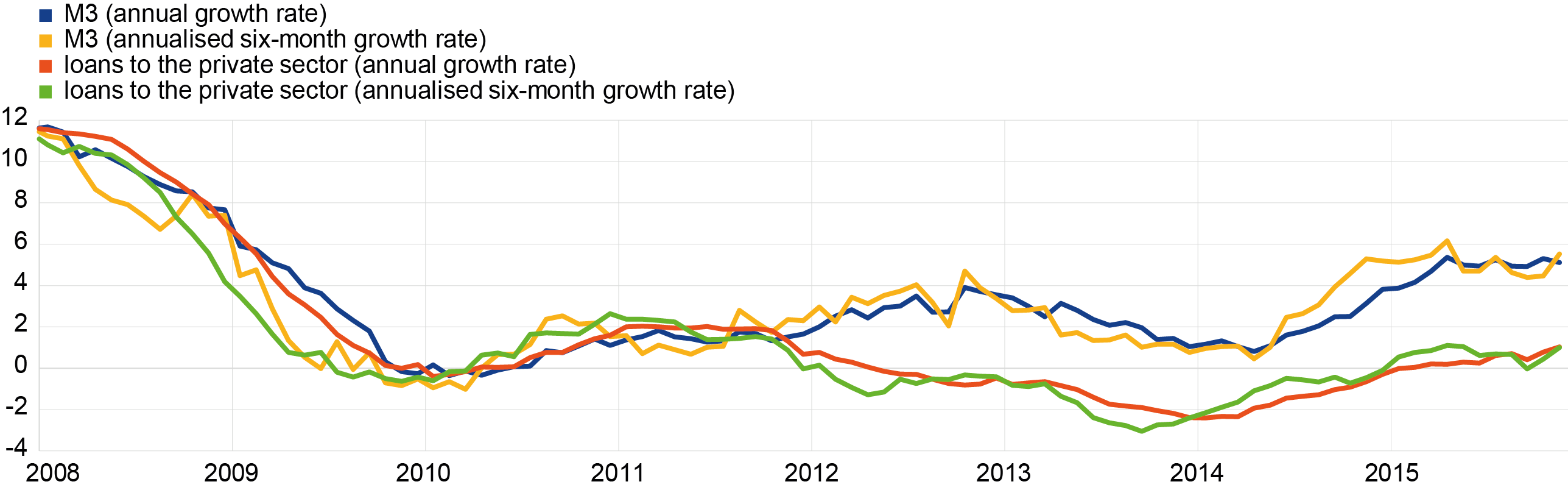
Source: ECB.
Note: The latest observation is for November 2015.
Overnight deposits continued to contribute strongly to M3 growth: the main factors behind this growth were the low opportunity costs of holding the most liquid components of money and the impact of the ECB’s expanded asset purchase programme (APP). By contrast, short-term deposits other than overnight deposits continued to contract, albeit to a lesser extent than in previous months. The growth rate of marketable instruments (i.e. M3 minus M2), which has a small weight in M3, remained positive, reflecting the recovery in money market fund shares/units observed since mid-2014 and the robust growth of monetary financial institution (MFI) debt securities in the money-holding sector with a maturity of up to two years. The said recovery in money market fund shares/units confirms market resilience to the negative interest rate environment.
Broad money growth was again mainly driven by domestic sources. From a counterpart perspective, the largest source of money creation in November was the bond purchases made by the Eurosystem in the context of the public sector purchase programme (PSPP). In addition, money creation continued to be supported by credit from MFIs to the euro area private sector and the reduction in the MFI longer-term financial liabilities (excluding capital and reserves) of the money-holding sector. This reflects the flatness of the yield curve, linked to the ECB’s non-standard monetary policy measures, which has reduced incentives to hold longer-term assets. It also highlights the Eurosystem’s purchases of covered bonds under the third covered bond purchase programme (CBPP3), which reduce the availability of such securities for the money-holding sector. Furthermore, the Eurosystem’s targeted longer-term refinancing operations (TLTROs), an alternative source of longer-term funding, have been curbing banks’ issuance activities. The contribution to annual M3 growth made by the MFI sector’s net external asset position remained negative. This reflects capital outflows from the euro area and is consistent with an ongoing portfolio rebalancing in favour of non-euro area instruments (there has been a lower appetite for euro area assets on the part of foreign investors). Euro area government bonds sold by non-residents under the PSPP account for the portfolio rebalancing.
Lending to the euro area private sector continued on a path of gradual recovery. [3] The annual growth rate of MFI loans to the private sector (adjusted for sales and securitisation) increased further in November (see Chart 9), with both loans to non-financial corporations (NFCs) and households accounting for the progress. Although the annual growth rate of loans to NFCs remained weak, it has recovered substantially from the trough of the first quarter of 2014. The ECB’s monetary policy measures and further easing of bank credit standards have supported this development. Despite these positive signs, the ongoing consolidation of bank balance sheets and persistently high levels of non-performing loans in some jurisdictions continue to hamper loan growth.
Chart 10
Composite bank lending rates for NFCs and households
(percentages per annum)

Source: ECB.
Notes: The indicator for the composite bank lending rates is calculated by aggregating short and long-term rates using a 24-month moving average of new business volumes. The latest observation is for November 2015.
Bank lending rates for NFCs and households remained broadly stable in November (see Chart 10). Despite recent signs of stabilisation, composite lending rates for NFCs and households have declined by significantly more than market reference rates since the ECB’s credit easing package was announced in June 2014. This development is related to receding fragmentation in euro area financial markets and the improvement in the pass-through of monetary policy measures to bank lending rates. Furthermore, the decline in composite lending rates has been supported by a decrease in banks’ composite funding costs, which stand at historically low levels. Between May 2014 and November 2015, the composite lending rate on loans to euro area NFCs fell by more than 80 basis points to 2.12%. And, over the same period, the composite lending rate on loans to households for house purchase decreased by more than 60 basis points, reaching 2.27% in November. Moreover, the spread between interest rates charged on very small loans (loans of up to €0.25 million) and those charged on large loans (loans of above €1 million) in the euro area decreased further in November. This indicates that small and medium-sized enterprises have benefited to a larger extent than large firms from the recent lending rate developments.
The January 2016 euro area bank lending survey (BLS) suggests that changes in credit standards and loan demand continue to support the recovery in loan growth (see survey at: https://www.ecb.europa.eu/stats/money/surveys/lend/html/index.en.html). In the fourth quarter of 2015, banks further eased (in net terms) credit standards for loans to NFCs. There was also a net easing of credit standards for loans to households for house purchase, marking a reversal from previous tightening. Increased competition remained the main factor driving less stringent credit standards. Net loan demand by NFCs and households rose considerably on the back of the low general level of interest rates. Financing needs related to working capital and fixed investment, consumer confidence and housing market prospects were additional factors behind stronger loan demand.
NFCs’ net issuance of debt securities rose modestly in November 2015. The turnaround in net issuance was supported by the observed temporary decline in the cost of market-based debt financing during November. By contrast, the ongoing strong growth of retained earnings has most likely been a dampening factor in recent months. Note that, in the third quarter of 2015, retained earnings still featured a double-digit annual growth rate.
The overall nominal cost of external financing for NFCs is estimated to have increased moderately in December 2015 and in the first half of January 2016. This rise is mainly explained by the higher cost of equity financing (there was a visible decrease in share prices), with the cost of debt financing remaining almost unchanged. In December 2015 and mid-January 2016 the cost of equity and market-based debt financing was, on average, around 40 and 20 basis points higher, respectively, than in November 2015.
Boxes
Box 1 What is driving Brazil’s economic downturn?
Following rapid economic growth in the years preceding the recent global financial crisis, Brazil was in a strong position to weather the Great Recession. Both the commodity price cycle and abundant capital inflows played a role in this improved economic performance. The improvement was also the result of the profound changes in macroeconomic policy management introduced a decade previously, with the end of fiscal dominance and hyperinflation in 1994. However, Brazil’s economic situation has deteriorated significantly in recent years. The economy entered into recession in 2014 and the situation worsened in 2015, with real GDP likely to have declined by 3%, while inflation has remained close to 10%. This box outlines the main factors underlying the economic slump in Brazil.
Chart A
GDP growth and major export commodity prices
(left-hand scale: index 2000=100; right-hand scale: annual percentage changes)
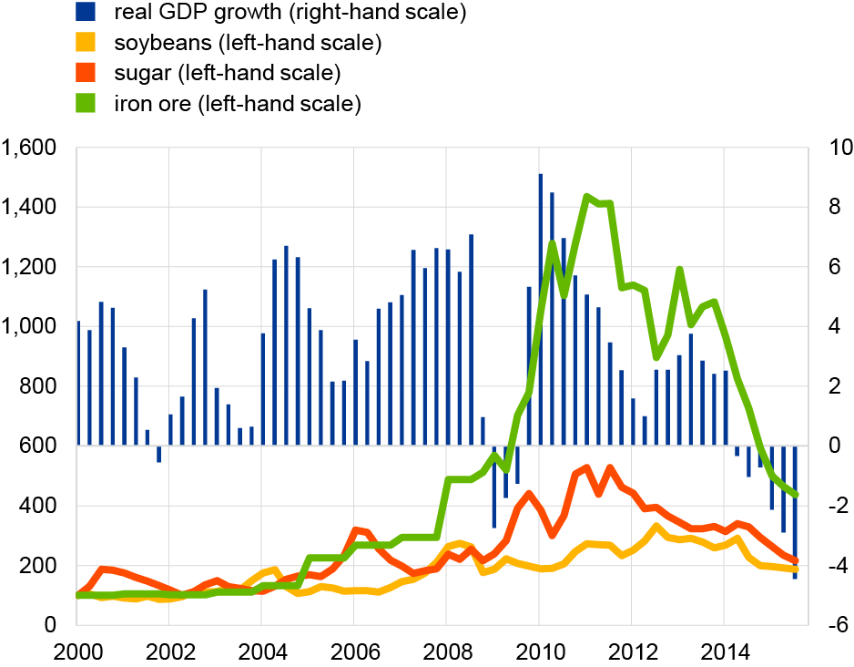
Sources: World Bank, CBOT – CME Group and IBGE – Instituto Brasileiro de Geografia e Estatistica.
The downturn of the non-energy commodity price cycle revealed the underlying structural weaknesses in the Brazilian economy. In the first decade of the century, Brazil benefitted from strong demand – particularly from China – for some of its key export commodities (e.g. iron ore, soybeans and raw sugar). Supported by positive terms of trade effects, Brazil’s annual GDP growth rate averaged 3.1% over this period. Since the fall in commodity prices in 2011 (see Chart A), these terms of trade effects have reversed. As a result, GDP growth has been consistently lower than predicted, while structural weaknesses underlying the economy have resurfaced. These weaknesses include a burdensome tax system, a sizeable informal sector, poor infrastructure, limited competition, the high costs of starting a business and high tariff rates.
Moreover, imbalances rose amid expansionary policies and strong capital inflows. Around the turn of the decade, Brazil continued to receive strong capital inflows, which amounted annually to around 9% of GDP. While these inflows kept sovereign and corporate spreads low, they fuelled a strong appreciation of the Brazilian real that hurt price competitiveness. Many companies, including large oil companies such as state-owned Petrobras, took advantage of the loose financing conditions to borrow on international markets to finance long-term investments. At the same time, monetary and fiscal policy was expansionary. The official interest rate was cut to a historic low of 7.25% in October 2012 (see Chart B), while subsidised public sector lending, coupled with a rise in tax exemptions to revive business confidence, sharply increased fiscal deficits. Given the lack of structural reforms, however, these measures led to only a moderate and temporary pick-up in GDP growth in 2012-13, while also contributing to rising inflation and a widening of the current account deficit (see Chart C).
Chart B
Inflation rate, overnight rate and real effective exchange rate
(left-hand scale: index 2006=100; right-hand scale: annual percentage changes)
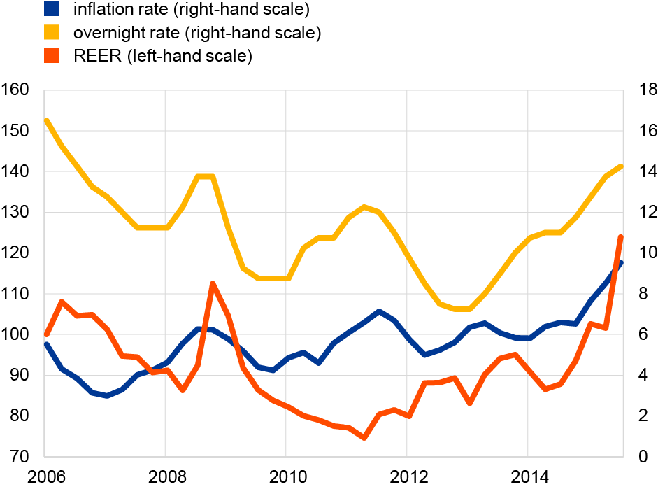
Sources: World Bank, CBOT – CME Group and IBGE – Instituto Brasileiro de Geografia e Estatistica.
Notes: The SELIC rate is the Brazilian Central Bank's overnight rate. REER stands for real effective exchange rate against 13 main trading partners; increasing values reflect a depreciation of the currency.
Chart C
Total public sector balance and current account balance (relative to GDP)
(percent of GDP, four-quarter moving averages)

Source: IBGE – Instituto Brasileiro de Geografia e Estatistica.
The shift in global financial market sentiment amid the US Federal Reserve’s announcement that it would wind down asset purchases (the “taper tantrum”) in May 2013 had a significant impact on the Brazilian economy. Global market sentiment suddenly turned against vulnerable emerging market economies with high external and fiscal imbalances, such as Brazil. Despite indications of an impending recession, monetary and fiscal policies were tightened in an attempt to restore macroeconomic credibility. In order to limit capital outflows and support the exchange rate, the Banco Central do Brasil raised its official interest rate to 14.25% in July 2015. On the fiscal front, limits on subsidised lending programs were cut and price subsidies were reduced. At the same time, however, the deterioration in global financial market conditions and the rise in interest rates entailed a surge in interest payments on public borrowing (to around 9% of GDP), which, in turn, raised gross public debt to historical highs (63% of GDP). As the country was unable to generate the fiscal surplus needed to stabilise debt with a sufficiently credible fiscal plan, two rating agencies downgraded Brazil from its investment grade rating for the first time in seven years. Notwithstanding the contraction of Brazilian GDP, inflation surged to over 10% in the last two months of 2015, owing to an adjustment of regulated prices and the sharp depreciation of the currency.
Model estimates suggest that the recent downturn in Brazil is, to a large extent, driven by a combination of domestic factors and lower commodity prices. According to the historical decomposition from a structural Bayesian VAR model[4] (see Chart D), the most significant factors in explaining the decline in Brazilian GDP since mid-2014 have been adverse commodity price developments and shocks to domestic factors, including domestic demand, monetary policy and financing costs. External shocks (defined as global uncertainty shocks and shocks to global financing conditions and foreign demand), on the other hand, have been less significant as a cause of the recent slowdown. In particular, the prices of iron ore and raw sugar – which account for 13% and 5% respectively of total exports – have been falling since 2011, while the price of oil – which accounts for 7% of total exports – has fallen since 2014. As Brazil is still a net oil importer, the main channel through which lower oil prices affect GDP is likely to be investment, rather than purely the terms of trade, as is the case for net oil exporting countries. Total investment has declined by 6% on average since early 2014, partly due to developments at Petrobras, the public oil producer, which accounts for 10% of total Brazilian investment and almost 2% of GDP. The company had to cut investment by 33% in both 2014 and 2015 to adjust to lower oil prices and also in response to a widespread corruption case, triggering confidence effects throughout the economy. The direct and indirect effects of the decline in investment by Petrobras have been estimated by Brazil's Ministry of Finance to have subtracted around 2 percentage points from GDP growth in 2015.
Chart D
Historical shock decomposition of annual real GDP growth
(left-hand scale: median estimates – deviation from long-run mean; right-hand scale: annual percentage changes)

Sources: IBGE – Instituto Brasileiro de Geografia e Estatistica and ECB staff calculations.
Note: Long-run mean refers to the period from the first quarter of 2000 to the second quarter of 2015.
Looking ahead, the risks facing Brazil remain on the downside amid uncertainties on fiscal policy and political difficulties which might further reduce confidence.
Box 2 A closer look at differences between industrial gross value added and industrial production
Industrial gross value added and industrial production are both very informative indicators of developments in industrial activity. Although conceptually similar, there are a number of differences between the two. [5] Looking at the data available for the latest two quarters, the weakness in euro area industrial production excluding construction in the second quarter of 2015 was not matched by weakness in the corresponding value added (quarterly growth rates were -0.1% versus 0.4%). In the third quarter of 2015, however, industrial production growth provided a more positive picture (growth of 0.2% versus 0.0% for value added). Against this background, this box takes a closer look at the differences between these two indicators for the euro area and explains the methodological differences that give rise to them. Industrial production is a short-term statistic that aims to estimate value added on a monthly basis in order to provide a timely measure of industrial activity. In practice, however, it is difficult to collect value added data on a monthly basis, which means that the monthly change in industrial production is typically derived from other sources, including deflated turnover, physical production data, labour input and intermediate consumption of raw materials and energy. Gross value added Looking at the data available for the latest two quarters, the weakness in euro area industrial production excluding construction in the second quarter of 2015 was not matched by weakness in the corresponding value added (quarterly growth rates were -0.1% versus 0.4%). In the third quarter of 2015, however, industrial production growth provided a more positive picture (growth of 0.2% versus 0.0% for value added). Against this background, this box takes a closer look at the differences between these two indicators for the euro area and explains the methodological differences that give rise to them. Industrial production is a short-term statistic that aims to estimate value added on a monthly basis in order to provide a timely measure of industrial activity. In practice, however, it is difficult to collect value added data on a monthly basis, which means that the monthly change in industrial production is typically derived from other sources, including deflated turnover, physical production data, labour input and intermediate consumption of raw materials and energy. Gross value added[6], on the other hand, is a quarterly national accounts indicator and is measured by subtracting intermediate consumption from output. Industrial production therefore only partly describes the development of industrial value added in terms of volume over a longer period, as the link between industrial production and value added may be affected by changes in input ratios and structures of production.
Movements in euro area industrial value added and production (excluding construction) differ in terms of absolute levels and quarterly growth rates. Chart A plots both indicators of euro area industrial activity in level terms. It shows that for euro area industry excluding construction, the level of value added has, for the most part, been higher than that of industrial production since 2000. This notwithstanding, both indicators tend to show similar cyclical movements in terms of quarter-on-quarter growth (see Chart B), but there have been marked differences of up to 2 percentage points, positive or negative, in some quarters since 2000. The difference between the two growth rates has been 0.1 percentage point on average since 2000. Looking at growth differences in absolute terms, the average as well as standard deviation has been 0.4 percentage point since 2000. This outcome implies that the differences in growth rates seen in the second and third quarter of 2015 were in a range one could expect.
Chart A
Level of euro area industrial value added and production (excluding construction)
(2000=100; gross value added: calendar and seasonally adjusted chain-linked volumes; industrial production index: quarterly average of working day and seasonally adjusted monthly data)

Sources: Eurostat and ECB calculations.
Chart B
Growth in euro area industrial value added and production (excluding construction)
(quarter-on-quarter growth rates; gross value added: calendar and seasonally adjusted chain-linked volumes; industrial production index: quarterly average of working day and seasonally adjusted monthly data; percentage points)
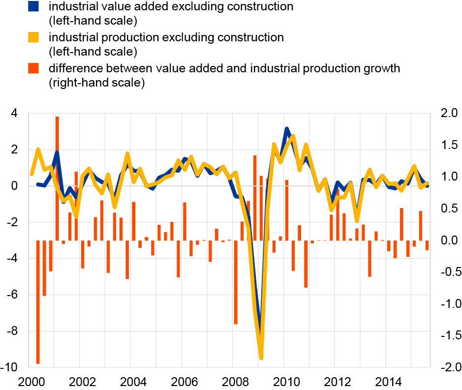
Sources: Eurostat and ECB calculations.
Differences in the movements of the two indicators also occur at the euro area country level, but to a varying degree. Among the four largest euro area countries, the difference between the quarter-on-quarter growth in industrial value added and industrial production (excluding construction) since 2000 has been greatest for Spain (0.4 percentage point), France (0.3) and Italy (0.2), but small for Germany (0.03). For five euro area countries this difference in growth over the same period has been negative, most markedly for Ireland and Luxembourg (both -0.6 percentage point). It should be borne in mind, however, that these results are also dependent on the period under investigation. For example, for Germany – where more historical data are available – the slight positive bias in growth rates for the period from 2000 turns slightly negative if the observation period starts in 1991.
In addition to conceptual factors, a number of other factors contribute to the differences between the two indicators, [7] such as seasonal adjustment on an infra-annual basis, as value added is adjusted at a quarterly frequency and industrial production at a monthly frequency. In order to quantify this factor, industrial production data were seasonally adjusted across euro area countries at a quarterly frequency. The outcome, which depends on the parameters applied for the seasonal filters, shows that quarterly growth rates can differ substantially depending on whether the seasonal adjustment is monthly or quarterly (see Chart C). Using data that are seasonally adjusted on a quarterly rather than a monthly basis, the average absolute difference between the growth rates of euro area industrial production is shown to have been 0.5 percentage point since 2000. On average, however, the impact of the other factors remains sizeable.
Chart C
The effects of seasonal adjustment on data measuring growth in euro area industrial production (excluding construction)
(quarter-on-quarter growth rates; percentage points)

Sources: Eurostat and ECB calculations.
Prices are treated differently in the two indicators. Gross value added is compiled using basic prices and does not include taxes (less subsidies) on products, whereas industrial production is at factor cost. The difference between value added at basic prices and at factor cost is other taxes (less subsidies) on production, figures for which are not available in volume terms at a quarterly frequency. In addition, whereas gross value added volumes are calculated using annual chain-linking, only a few countries so far apply this for industrial production.
Different economic activities are included in the two indicators. Value added includes water supply, sewerage, waste management and remediation activities (Section E[8]), whereas industrial production does not. The share of this activity in industrial value added excluding construction since 2000 has varied between 4.2% in 2007 and 5.0% in 2009. Chain-linked volume value added series for this sector are only published at an annual frequency and are rather acyclical. Calculations breaking down these annual data into quarterly data indicate that the quarter-on-quarter difference in the growth rate of industrial value added and production remains, on average, at a similar magnitude. Nevertheless, for specific quarters, the impact of Section E is found to be sizeable, i.e. up to 2.2 percentage points during the Great Recession and up to 0.8 percentage point during “normal” times.
A further source of difference between the two indicators is that industrial production typically covers firms above a certain threshold (in terms of turnover or number of employees), with thresholds varying across countries. National accounts attempt to provide a more complete picture by using data from a variety of alternative sources.
All in all, despite the close link between value added and industrial production, the differences between the two indicators reflect all of the above-mentioned factors to some degree, although their relative importance is difficult to assess. From an economic perspective, it is useful to monitor both indicators to assess the economic status of industrial activity. Further harmonisation between national accounts and short-term statistics, as well as between national practices for seasonal adjustment, would help to reduce these differences.
Box 3 Eurosystem publishes more detailed criteria for accepting rating agencies
The Eurosystem has published more detailed criteria that rating agencies must meet to be part of its framework for mitigating financial risk in monetary policy operations. The Eurosystem credit assessment framework or ECAF defines the minimum credit quality requirements that ensure the Eurosystem accepts only assets with high credit standards as collateral. The Eurosystem has a legal obligation to lend money only against adequate collateral.[9] The ECAF also forms the basis of minimum credit quality requirements in the context of outright purchases.
Rating agencies are one source of information in the framework. [10] When rating agencies are accepted under the framework as When rating agencies are accepted under the framework as “external credit assessment institutions” or ECAIs, their ratings are used mainly to assess the credit quality of marketable assets (traded debt instruments, in particular bonds). Rating agencies can also be accepted under the framework as providers of rating tools. In addition, the Eurosystem u“external credit assessment institutions” or ECAIs, their ratings are used mainly to assess the credit quality of marketable assets (traded debt instruments, in particular bonds). Rating agencies can also be accepted under the framework as providers of rating tools. In addition, the Eurosystem uses information from in-house credit assessment systems and counterparties’ internal ratings-based systems. The last three types of credit assessment system are used mainly to assess non-marketable collateral such as credit claims. To ensure that the information provided by all four sources is conses information from in-house credit assessment systems and counterparties’ internal ratings-based systems. The last three types of credit assessment system are used mainly to assess non-marketable collateral such as credit claims. To ensure that the information provided by all four sources is consistent, accurate and comparable, the Eurosystem has established acceptance criteria for each credit assessment source, as well as a harmonised rating scale, against which it regularly monitors the performance of all accepted systems. These procedures aim to protect the Eurosystem against financial sistent, accurate and comparable, the Eurosystem has established acceptance criteria for each credit assessment source, as well as a harmonised rating scale, against which it regularly monitors the performance of all accepted systems. These procedures aim to protect the Eurosystem against financial risks as well as to ensure a level playing field among the credit rating providers.risks as well as to ensure a level playing field among the credit rating providers.
In December 2015 the Governing Council decided to publish further details on the criteria for accepting a rating agency into the ECAF. [11] The published criteria refer to the acceptance of rating agencies as external credit assessment institutions. An agency must, at the time of its application, be providing minimum coverage of assets eligible for use in monetary policy operations in terms of rated assets The published criteria refer to the acceptance of rating agencies as external credit assessment institutions. An agency must, at the time of its application, be providing minimum coverage of assets eligible for use in monetary policy operations in terms of rated assets[12], rated issuers and the volume of assets rated. The rating agency’s coverage must be diversified across the eligible asset classes and across euro area countries. For example, it must rate at least three of the four eligible non-public sector asset classes (covered bonds, uncovered bonds, corporate bonds and asset-backed securities) in two-thirds of the countries. In each asset class it must provide ratings for at least 10% of the eligible assets, 10% of the issuers and 20% of the nominal volume. Moreover, in the three years prior to its application the rating agency must have complied with these criteria at a level of at least 80%.
The requirements are designed to ensure that rating agencies have broad credit risk expertise and a track record over time. For efficiency reasons and in order to ensure that only rating agencies with established and broad credit risk expertise are accepted, the requirements take into account market acceptance of rating agencies’ ratings, the credit risk interlinkages[13] among the eligible asset classes, and the geographical concentration of eligible collateral in the euro area. At the same time, the thresholds are not so restrictive as to preclude the acceptance of new rating agencies: a rating agency assessing around 100 issuers, for example, may comply with the requirements, depending on the geographical and asset-class focus of its business.[14] Furthermore, the set of coverage criteria as a whole is designed to ensure that the Eurosystem has information to ascertain whether a rating agency has an adequate performance track record and to map its ratings to the harmonised rating scale. In addition, the 80% historical coverage requirement over the three years preceding an application allows new rating agencies to benefit from a gradual increase in their European coverage in order to apply to be accepted into the ECAF once they can demonstrate well-established broad credit risk expertise and proven market acceptance.
In the acceptance procedure, the Eurosystem investigates all additional information relevant for risk protection and the efficient implementation of the ECAF. [15] Compliance with the minimum coverage criteria serves only as a prerequisite for the initiation of an acceptance procedure. In view of the importance of the credit quality information for asset eligibility and valuation haircuts, the Eurosystem forms its decision on whether to accept a rating agency on the basis of a comprehensive due diligence assessment. Rating agencies must meet a number of information, regulatory and operational requirements. To be part of the framework they must, for example, be supervised by the European Securities and Markets Authority (ESMA). Furthermore, information on their credit ratings needed to monitor rating quality must be available to the Eurosystem. For efficiency purposes and in view of the resource-intensive due diligence process for each individual rating agency, the Eurosystem requires the minimum coverage criteria to be met before it considers accepting a new rating agency.
In addition, the Eurosystem is reinforcing its due diligence to avoid mechanistic reliance on external ratings. It is carrying out additional work to better understand the ratings, rating processes and methodologies of the rating agencies accepted in the ECAF. This is in line with various initiatives by international authorities aimed at reducing over-reliance on external ratings in legal, regulatory and other public frameworks.[16] In parallel, the Eurosystem has enhanced its internal credit assessment capabilities, for example by increasing the number of in-house credit assessment systems for non-financial corporations In parallel, the Eurosystem has enhanced its internal credit assessment capabilities, for example by increasing the number of in-house credit assessment systems for non-financial corporations[17] and by establishing a due diligence process in the context of the asset-backed securities and covered bond purchase programmes. and by establishing a due diligence process in the context of the asset-backed securities and covered bond purchase programmes.
Articles
Article Recent developments in the composition and cost of bank funding in the euro area
Changes in the composition and cost of bank funding have important implications for the provision of credit and, consequently, for economic output and inflation. Banks’ funding costs are affected by monetary policy, but the transmission of policy depends on many factors, including the strength of banks’ balance sheets and the macroeconomic environment. Therefore, developments in bank funding can be different across euro area banks and countries. This article gives an overview of recent developments in the composition and cost of bank funding, including capital, and shows that they varied across the euro area over the period of the financial crisis, which had an impact on the transmission of monetary policy. The interaction between monetary policy measures (both standard and non-standard) and banks’ funding conditions is also discussed.
Introduction
During the financial crisis, a large degree of heterogeneity in the cost of bank credit was linked to a divergence in funding conditions across euro area banks. Understanding banks’ funding conditions is vital for the analysis of credit provision to the real economy and, consequently, of output and inflation, particularly in the light of the fact that funding cost dynamics diverged from monetary policy rates during the crisis.[18] In general, banks seek funding from retail and wholesale sources. Retail funding, i.e. deposits from the private sector, is generally the dominant source of funding, and deposits from the non-financial private sector tend to be less volatile than wholesale funding sources, particularly when protected by deposit guarantee schemes. However, the importance of such sources for a bank’s overall funding depends on institutional features such as the bank’s size or business model. For small euro area banks, in particular, retail deposits account for a considerably larger share of overall funding than wholesale sources.[19] Wholesale funding includes interbank liabilities, which are used for short-term liquidity management, and the issuance of debt securities. Finally, banks also have access to central bank liquidity and raise capital, normally in the form of equity.
A well-functioning banking sector is essential for the effective transmission of monetary policy. This applies in particular to the euro area, where banks play a dominant role in providing external financing to the non-financial private sector. The outbreak of the financial and sovereign debt crisis in 2010 affected all segments of the financial system, especially the banking sector, which hampered the transmission of the ECB’s monetary policy measures to bank funding and, ultimately, to bank lending conditions. Moreover, bank funding conditions were heterogeneous across euro area countries in an environment of sluggish economic activity, high sovereign debt and concerns about weak banks. While differences in funding costs are to be expected, high levels of uncertainty led to excessive risk premia in some jurisdictions and there were periods when banks’ access to wholesale and, to a lesser extent, retail funding was severely hampered. At the same time, the ECB’s non-standard monetary policy measures (such as the policy of full allotment of the liquidity demanded by banks at a fixed rate and the two three-year longer-term refinancing operations (LTROs) in late 2011 and early 2012) acted as a strong backstop and prevented a disorderly and forced deleveraging that would have had a considerable negative impact on the overall economy. Since then, steps towards banking union, the ECB’s credit easing package announced in mid-2014, and the expanded asset purchase programme (APP) announced in early 2015 have led to a significant improvement in bank funding conditions, which have become more homogeneous across countries. This has helped to weaken the bank-sovereign nexus, thereby considerably reducing impairments in the transmission mechanism.
The funding and capital structures of banks are of interest for a number of reasons. The determinants of banks’ funding and capital structures are distinct from those of non-financial corporations.[20] Banks are subject to capital regulation because of the significant effect they can have on financial stability and economic growth: given that they are largely funded by deposits, a significant share of which are covered by guarantee schemes, banks are required to hold minimum amounts of capital to absorb losses and mitigate moral hazard concerns.[21] While this implies that the relative cost of equity and debt funding is not the main determinant of banks’ capital structures, it does not mean that their cost is irrelevant. In fact, the cost of capital is an important factor in banks’ portfolio allocation decisions, including lending activity. Recent developments in the European supervisory, regulatory and resolution framework – including macroprudential capital buffers, total loss-absorbing capacity (TLAC) requirements and the Bank Recovery and Resolution Directive (BRRD) – help to rectify incentives that are misaligned because of the expectation of public support (the too-big-to-fail problem). The effect of these measures on banks’ cost of funding is a priori unclear, as the direct effect of a reduction in implicit public sector support is at least partially offset by decreased risk-taking by banks. While the transition to the revised regulatory framework may constrain lending in the short term, it is expected to increase economic welfare in the medium to long term, as the negative externalities associated with systemic crises are contained.[22]
This article is structured as follows: Section 2 presents the main developments in the composition of banks’ funding and capital structures and discusses the monetary policy measures that have had an impact on funding quantities, Section 3 discusses developments in the cost of funding and capital and the impact of certain monetary policy measures on these costs, and Section 4 concludes.
The composition of funding and the impact of monetary policy
The structure of banks’ funding and capital is integral to the overall stability and cost of funding. During the crisis, there were changes not only in banks’ overall funding levels, but also in the structure of their funding. This section discusses some of the main changes in euro area banks’ funding over the past decade and compares developments in vulnerable and less vulnerable countries.[23] Banks are defined here as credit institutions and other monetary financial institutions (MFIs) that are resident in the euro area. The impact of monetary policy measures on funding quantities and composition is also discussed.
The composition of euro area banks’ funding has fluctuated over the past decade, reflecting changes in economic conditions, uncertainty and the monetary policy response to the crisis. Banks’ overall funding grew in line with the expansion in their assets until the escalation of the financial crisis following the collapse of Lehman Brothers and the resulting increase in uncertainty in interbank markets. Chart 1 shows annual flows in the main liabilities of MFIs, including capital. Funding flows increased steadily from 2005 until the end of 2007, particularly via wholesale funding sources, which include external (non-euro area) liabilities, interbank funding and shorter-term debt securities and tend to be more volatile than retail deposit funding. While growth in these wholesale funding sources facilitated the fast expansion of banks’ balance sheets in the years leading up to the crisis, the outflows and swift withdrawals observed at the start of the crisis made a significant contribution to bank funding pressures and a reduction in liquidity. Increased reliance on these funding sources is likely to have introduced a pro-cyclical bias in financial intermediation.[24]
Chart 1
Developments in funding of MFIs other than the Eurosystem
(EUR billions; annual flows by quarter)

Sources: ECB and ECB calculations.
Notes: The chart highlights three periods: 1. the collapse of Lehman Brothers, 2. the announcement of OMTs, and 3. the introduction of the credit easing package. The analysis is based on aggregate MFI data: deposits from other MFIs include operations between banks belonging to the same economic group. The components constitute MFIs’ main liabilities and exclude money market fund shares/units and remaining liabilities, which are composed mostly of derivatives. Data are annual flows starting in the first quarter of 2005 and ending in the third quarter of 2015. Deposits of MFIs include both interbank funding and funding from the Eurosystem.
Deposits from resident non-MFIs, and deposits from the non-financial private sector in particular, are the most stable and single largest component of funding for euro area banks. While the composition of these deposits varies across countries and bank types, they are the predominant source of funding for banks in both vulnerable and less vulnerable countries.[25] Retail deposits tend to be a more stable source of funding than wholesale sources:[26] since the liquidity services banks provide to depositors can incur transaction and switching costs, retail deposits are less susceptible to unanticipated withdrawals.[27] Moreover, as withdrawals are based on individual liquidity needs they tend to be more predictable, on the basis of the law of large numbers. In addition, deposits are generally insured up to a limit and are less subject to adverse shocks related to uncertainty.
As the financial crisis intensified with the collapse of Lehman Brothers, deposit flows fell, but remained robust relative to the other, more volatile sources of funding in both vulnerable and less vulnerable countries. Since changes in deposit levels are associated with changes in income and general economic conditions, the reduction in flows reflected, at least in part, the deterioration in the macroeconomic environment across the euro area.[28] As the sovereign debt and financial market stress intensified, deposit outflows became more pronounced in vulnerable countries, driven largely by a repatriation of funds by non-domestic depositors (both from other euro area countries and from outside the euro area). After reaching a peak in mid-2012, deposit outflows from vulnerable countries subsided and fragmentation in funding across the euro area receded. This can be explained largely by the ECB’s announcement of Outright Monetary Transactions (OMTs) and the decision taken at the June 2012 euro area summit by European leaders to deepen European integration in accordance with the long-term objective of creating a banking, fiscal and political union, as well as the decision to launch the Single Supervisory Mechanism (SSM).[29] While deposit flows in vulnerable countries recovered following these announcements, they remained weak relative to pre-crisis levels and then began to decline in an environment of low inflation and subdued income growth. Following the introduction by the ECB of further credit easing measures in the middle of 2014 and the announcement of the expanded APP at the beginning of 2015, deposit flows improved in an environment of increased central bank liquidity.
The sources of wholesale market funding that had increased in the years preceding the collapse of Lehman Brothers decreased rapidly at the start of the crisis, with debt securities issuance and interbank activity in particular slumping (see Chart 1). In vulnerable countries, as interbank funding deteriorated, banks continued to issue securities. A proportion of these were covered by government guarantees, whose aim was to support bank funding over this period.[30] However, issuance diminished as uncertainty and fears regarding the solvency of sovereigns increased. While market risks receded in the middle of 2012, there was a second stage of negative net issuance of debt securities by banks at this time, partly reflecting the correction of excessive leverage of the financial and non-financial sectors, as well as a move towards a more comprehensive regulatory and supervisory framework. Moreover, debt securities funding was replaced by Eurosystem liquidity because the cost of the latter was more favourable. Overall deposit flows from MFIs, which include interbank and Eurosystem funding, decreased as the financial crisis intensified (see Chart 1). Crucially, however, the composition of the deposits changed as more volatile interbank liquidity was partially replaced by central bank liquidity (see Chart 2). Interbank liquidity grew in the years before the financial crisis, reflecting increased international interlinkages among banks as cross-border lending increased over time. With the collapse of Lehman Brothers, the use of interbank deposits as a short-term liquidity tool decreased in line with a need to deleverage and amid general uncertainty about the creditworthiness of counterparties.[31]
Chart 2
Breakdown of MFI deposits at MFIs other than the Eurosystem
(EUR billions; monthly outstanding amounts)

Source: ECB.
Note: The series for the Eurosystem comprises its lending to euro area credit institutions related to monetary policy operations denominated in euro and other claims on euro area credit institutions denominated in euro.
The financial market stress not only resulted in a shift towards Eurosystem liquidity and away from interbank liquidity, particularly in vulnerable countries (see Chart 2), there was also a change in the composition of the Eurosystem liquidity, largely owing to the monetary policy response to the crisis. [32] At the start of the crisis the ECB switched to a fixed rate full allotment tender procedure whereby, as long as banks had adequate collateral, their liquidity demands were fully satisfied at a rate determined by the Governing Council, which provided certainty and stability to the banking sector.[33] Moreover, the maturity of the liquidity was extended by means of LTROs.[34] As the sovereign debt tensions intensified and concerns about bank solvency increased, the ECB announced two three-year LTROs, the first of which took place at the end of 2011 and the second at the start of 2012. The share of outstanding Eurosystem liquidity in banks’ funding increased substantially following these operations, reaching its highest level around the middle of 2012. There is evidence that these operations bolstered the supply of bank credit and, consequently, output and inflation over the crisis.[35] As part of a credit easing package introduced in June 2014, the ECB also announced a series of targeted LTROs (TLTROs), providing liquidity with a maturity of up to four years and linked to banks’ lending volumes, in order to enhance the functioning of the monetary policy transmission mechanism by supporting the provision of credit to the real economy.[36] The weighted average maturity of bank borrowing from the Eurosystem increased from around 130 days before the first TLTRO was conducted to around 800 days after the settlement of the fifth TLTRO in September 2015.[37] In the July 2015 euro area bank lending survey, banks reported that the TLTROs had improved and were likely to further improve their liquidity position, market financing conditions and profitability, and that they had been and would be used as a substitute for other funding sources, mainly other Eurosystem liquidity operations, maturing debt and interbank lending.[38] The Eurosystem also changed the collateral framework during the crisis, mainly by expanding the list of assets eligible as collateral in monetary policy operations and by lowering the rating required on assets. The Eurosystem also changed the collateral framework during the crisis, mainly by expanding the list of assets eligible as collateral in monetary policy operations and by lowering the rating required on assets.[39] These changes were essential for the functioning of the banking system, particularly when stress in sovereign markets led to rating downgrades. They ensured that solvent banks could still access liquidity, in order to prevent an escalation of the crisis.[40] During the crisis, banks used their highest quality collateral for direct repo transactions in the wholesale markets, while non-marketable collateral was increasingly posted with the Eurosystem (see Chart 3).
Chart 3
Use of collateral
(EUR billions after valuation and haircuts)

Source: ECB.
Notes: Averages of month-end data over each period.* Since the first quarter of 2013 the category “non-marketable assets” has been split into two categories: “fixed-term and cash deposits” and “credit claims”.
During the crisis, in addition to the decline in the overall level of interbank liquidity, there was a change in its composition, reflecting perceptions of increased counterparty risk. There was a considerable move from unsecured to secured lending, particularly from 2008 onwards (see Chart 4), as well as a substantial adjustment in activity towards domestic counterparties and away from counterparties from other euro area countries.[41] Concerns about counterparty creditworthiness resulted in increased use of central counterparties, which facilitate clearing and settlement in money markets by acting as the direct counterparty for both lender and borrower, thereby assuming the risk of the borrower defaulting.[42]
Chart 4
Euro area money market volumes
(annual indices, 2005=100)

Source: ECB.
External liabilities increased substantially in the years preceding the crisis and facilitated the growth in banks’ balance sheets. However, in the wake of the Lehman Brothers collapse there was a swift contraction in external liabilities, partly owing to asymmetric information and a sudden rise in risk aversion among international investors.[43] The growth in external liabilities in the lead-up to the crisis stemmed from deposits of non-euro area residents and holdings by non-residents of shorter-term debt securities issued by euro area banks, and largely reflected the expansion of cross-border interbank liquidity (see Chart 1). This facilitated the growth in banks’ balance sheets, as deep and liquid cross-border financial markets eased quantitative constraints on their liquidity management. However, at the outbreak of the crisis, cross-border funding was withdrawn quickly, which increased banks’ exposure to adverse global funding pressures.[44] For vulnerable countries, external liability flows have remained broadly negative since the onset of the crisis. For less vulnerable countries, annual flows have increased recently, and have been generally positive since the ECB’s announcement of additional monetary policy easing measures in the middle of 2014.
Chart 5
Capital and reserves of euro area MFIs other than the Eurosystem
(percentages of total assets)

Source: ECB.
Note: Total assets, capital and reserves were derived via notional stocks in order to avoid reclassifications, revaluations and changes in the composition of the euro area impacting on this measure.
The adverse changes in prices and credit losses associated with the crisis led to impairments in banks’ capital positions, which, in conjunction with funding pressures, often necessitated deleveraging and changes in banks’ liabilities, such as increased capital issuance. Chart 5 shows that capital as a percentage of total assets was relatively stable in the pre-crisis period. The subsequent increase in the ratio was particularly pronounced for banks in vulnerable countries, where levels of assets decreased and levels of capital increased in response not only to regulatory requirements but also to pressure from markets to hold larger discretionary buffers against losses. Over this period, in addition to the capital raised in private sector markets, a substantial amount of capital was also obtained through government capital injections.[45] The Capital Requirements Directive and Regulation (CRD IV/CRR), which came into force in January 2014, increased both the quality and the amount of capital that banks must hold for prudential purposes. In addition, new European legislation has set the stage for the creation of a banking union and addressed gaps in the capital framework that were highlighted by the crisis.
Over the past decade the funding structure of euro area banks has been altered by changes in market risk, the economic environment and monetary policy measures: there is now a greater reliance on more stable funding relative to volatile funding. [46] Table shows that MFIs’ increased reliance on deposit funding and decreased reliance on debt securities and external liabilities is common to both vulnerable and less vulnerable countries. The table also shows the breakdown in MFI deposits between interbank and Eurosystem liquidity, illustrating the fact that while the decrease in interbank liquidity has been a general phenomenon across the euro area, it has been greatest in vulnerable countries. Reliance on central bank liquidity grew between January 2005 and September 2015 in vulnerable countries, in contrast to the situation in less vulnerable countries. The nature of interbank liquidity has also changed from unsecured to secured (see Chart 4), and there has been a reduction in the reliance on cross-border activities, including with non-euro area counterparties (reflected in the reduced relevance of external liabilities). Vulnerable countries in particular now have a substantially larger share of capital in total funding. While this measure of capital differs from the regulatory measure, its increase follows a general improvement in solvency and leverage ratios.[47] Overall, these changes indicate a move towards a business model with a greater reliance on more stable funding sources.[48]
The structure of banks’ balance sheets and funding will continue to be affected by the economic and policy environment, and in particular by the expanded APP, which will inject further liquidity into the banking system. The expanded APP, which comprises two private sector asset purchase programmes (the asset-backed securities purchase programme (ABSPP) and the third covered bond purchase programme (CBPP3)) and the public sector purchase programme (PSPP), aims to ease financing conditions and bring the path of inflation back in line with price stability.[49] The APP has had a substantial impact on banks The APP has had a substantial impact on banks’ balance sheets: as the Eurosystem pays for the assets it purchases by supplying reserves, purchases are always settled through banks regardless of who the ultimate seller is. In terms of funding, increases in reserves following the introduction of the expanded APP have so far been reflected larg’ balance sheets: as the Eurosystem pays for the assets it purchases by supplying reserves, purchases are always settled through banks regardless of who the ultimate seller is. In terms of funding, increases in reserves following the introduction of the expanded APP have so far been reflected largely in increases in deposits (see Chart 6), which partly reflect banks’ intermediation of bond sales to the Eurosystem by euro area non-banks. The sizeable decline in net external assets reflects the intermediation of sales by non-euro area residents. Credit to governments has declined, which, at ely in increases in deposits (see Chart 6), which partly reflect banks’ intermediation of bond sales to the Eurosystem by euro area non-banks. The sizeable decline in net external assets reflects the intermediation of sales by non-euro area residents. Credit to governments has declined, which, at least partly, reflects sales of securities to the Eurosystem from banks’ own portfolios and contributes to the increase in reserves. Chart 6 also shows an increase in credit to the private sector, part of which will have contributed to the above-mentioned increase in deposits. least partly, reflects sales of securities to the Eurosystem from banks’ own portfolios and contributes to the increase in reserves. Chart 6 also shows an increase in credit to the private sector, part of which will have contributed to the above-mentioned increase in deposits.
Table
Structure of main liabilities of euro area MFIs other than the Eurosystem
(percentages of main liabilities)

Source: ECB.
Notes: The main liabilities consist of total liabilities excluding remaining liabilities, and shares/units issued by money market funds. Remaining liabilities consist of volatile components that are separate from the core activities of banks, including in particular (negatively-valued) financial derivatives, for which there are some variations in accounting and statistical treatment over the period under review and across jurisdictions.
Chart 6
Movements in the balance sheet of MFIs other than the Eurosystem that correspond to the change in reserve holdings between end-February and end-September 2015
(EUR billions; non-seasonally adjusted)

Sources: ECB and ECB calculations.
Notes: Increases in net asset positions reduce claims on the Eurosystem; increases in net liability positions increase claims on the Eurosystem. “Wholesale funding (net)” refers to issuance of debt securities net of holdings of MFI debt securities, and borrowing from MFIs other than the Eurosystem net of deposits with MFIs other than the Eurosystem.
Chart 7
Impact of the APP on euro area banks’ profitability and capital position, as reported in the April and October 2015 bank lending surveys
(net percentages of respondents)

Source: ECB.
Notes: Impact over the past six months. The net percentages are defined as the difference between the sum of the percentages of banks responding “increased/improved considerably” and “increased/improved somewhat” and the sum of the percentages of banks responding “decreased/deteriorated somewhat” and “decreased/deteriorated considerably” to the corresponding question in the April and October 2015 bank lending surveys. The results shown are calculated as a percentage of the number of banks that did not reply “not applicable”.
According to the April and October 2015 bank lending surveys, the contribution of the APP to euro area banks’ profitability and solvency positions has been positive overall, even though the effects are varied and differ across countries (see Chart 7). Although the APP has led to capital gains associated with the valuation of securities held by banks, its effect on net interest income is a priori unclear. On the one hand, the compression of yields and the flattening of the yield curve have led to lower interest income. This is likely to translate into lower unit margins, since liabilities tend to have shorter maturities than assets and are less responsive to decreasing interest rates, particularly when they are at very low levels. Furthermore, the APP generates excess liquidity which, if deposited with the Eurosystem, is remunerated at a negative rate. On the other hand, these effects are at least partly offset by the increased intermediation activity and credit quality stemming from the programme’s positive impact on output. The APP has made a modest contribution to bank profitability in the euro area as a whole, but its impact has been positive for vulnerable countries in particular. For the euro area aggregate, the estimated negative effects on net interest income have so far been outweighed by the positive effects from capital gains and improved credit quality against the background of the APP’s positive impact on economic activity. The effect on the capital ratio has also been positive, although the effects have diminished since the initial announcement and implementation of the programme.
The cost of funding and the effects of monetary policy
As the financial crisis escalated, stress in financial markets caused the cost of funding for many euro area banks to increase. Uncertainty regarding the health of certain banking markets led not only to outflows, but also to increases in risk premia on the funds available to banks. Wholesale funding sources became either unavailable or prohibitively expensive for many banks in vulnerable countries, leading to an increase in recourse to central bank operations, as outlined in Section 2. The observed market fragmentation reflected high uncertainty and risk aversion and was at times greater than would be expected given the actual underlying risks. Since the degree of dispersion in lending rates and heterogeneity in the transmission of monetary policy were salient features of the crisis, this section uses data at both the country and the bank level to explore movements in the level and dispersion of the different funding elements over time. These data contain detailed information on quantities of deposits held by the non-financial private sector, debt securities issued by banks and capital, as well as prices of deposits and securities and an estimate of the cost of equity.
The cost of deposits across euro area countries can vary for a number of reasons, such as differences in maturity or market structure and variation in credit risk and in institutional factors, including regulation and taxation. [50] Despite these differences, the transmission of monetary policy must be smooth across euro area countries and banks in the long run. Uncertainty and stress in the financial markets during the crisis meant that credit risk concerns fuelled financial market fragmentation and hindered transmission as dispersion in pricing behaviour across banks increased in relation to the perceived interaction with sovereign credit risk in their country of residence.[51]
Chart 8
Composite euro area bank deposit rates for the non-financial private sector
(percentages per annum)

Source: ECB.
Note: Composite rates are computed as averages of new business rates for different maturities, weighted by outstanding amounts.
Developments in deposit rates have broadly followed monetary policy rates, albeit with an incomplete pass-through. As the interest rate on the ECB’s main refinancing operations (MROs) was cut from 4.25% at the end of September 2008 to 1.00% in May 2009, deposit rates in the euro area also fell, although to a lesser extent (see Chart 8). In October 2008 they stood at around 2.95%, and reached a trough of around 1.0% at the beginning of 2010. From the middle of 2010, deposit rates started increasing gradually and, following two policy rate increases in the middle of 2011, stood at around 1.45% at the end of 2011. Monetary policy then resumed an easing cycle, whereby the MRO rate was cut incrementally from 1.50% in November 2011 to 0.05% in September 2014. Deposit rates fell over this period, and the average composite rate currently stands at around 0.4%. Moreover, the dispersion of deposit rates has narrowed somewhat, as they are close to the zero lower bound, particularly for shorter maturities. However, the number of banks with negative deposit rates for any segment remains small (see Chart 10).
Before the crisis deposit rates were lower overall in vulnerable countries than in less vulnerable countries. This is largely explained by the difference in the maturity of the deposits (see Chart 9). Particularly in vulnerable countries, overnight deposits made up a significant share of bank deposits from the non-financial sector. Since the crisis, the share of overnight deposits has increased in both vulnerable and less vulnerable countries against the background of lower interest rates. However, the increase in the weight of overnight deposits started later in vulnerable countries, against a background of hampered access to wholesale funding markets. The share of long-term deposits has declined somewhat in the euro area as a whole, driven by developments in less vulnerable countries, but it remains considerably higher than in vulnerable countries.
Chart 9
Breakdown of non-financial private sector deposits by maturity
(EUR billions)

Source: ECB.
Deposit rates in vulnerable countries did not fully follow policy rate declines at the height of the crisis. The median deposit rate for banks in vulnerable countries fell from 2.86% in September 2008, when policy rates were cut, to around 1.15% in mid-2012 (see Chart 10).
Chart 10
Distribution of euro area bank deposit rates for the non-financial private sector
(percentages per annum)

Sources: iBoxx and ECB.
Notes: Composite rates are computed as averages of new business rates for different maturities, weighted by outstanding amounts. The chart shows the density approximation of the distribution of deposit rates obtained from a sample of MFIs in vulnerable and less vulnerable countries.
In less vulnerable countries, the median deposit interest rate fell further (from 3.58% to 0.88%). In vulnerable countries, deposit outflows and banks’ need to attract more stable funding may have stemmed the decrease in rates.[52] Since the OMT announcement in the middle of 2012, deposit outflows linked to concerns about the health of sovereigns and banks have receded. Deposit rates have fallen and the dispersion in pricing across banks in vulnerable countries has also declined notably, particularly following the announcement of further credit easing by the ECB in mid-2014 and the expanded APP in early 2015. Deposit rates are increasingly clustered at zero as the effect of monetary easing keeps funding costs low. Nonetheless, banks have proved reluctant to set negative deposit rates. This is likely to reflect commercial policies, since retail depositors are likely to be less averse to an increase in commissions than to a negative deposit rate. It may also reflect the gradual pass-through of past cuts in monetary policy rates to deposit rates and the recent re-pricing in wholesale markets.
Chart 11
Yields on bonds issued by euro area banks
(percentages per annum)

Sources: iBoxx and ECB.
Note: Bank bond yields are averaged by outstanding amount of securities issued.
Banks’ access to market funding deteriorated during the crisis, with funding flows diminishing and the cost of issuing debt securities increasing substantially. Around the time of the turmoil related to the sub-prime mortgage crisis in the United States and the collapse of Lehman Brothers there was a general increase in market funding costs in the euro area (see Chart 11). While this increase was more significant in vulnerable countries, it was driven by a small number of large banks that were particularly affected by the collapse of Lehman Brothers. When the sovereign debt crisis broke out in early 2010, the level and dispersion of market funding costs increased in vulnerable countries, while banks in less vulnerable countries were more insulated from the turmoil. By the middle of 2011, as the sovereign debt crisis intensified, market funding costs for banks in both vulnerable and less vulnerable countries had increased, although the gap between them also widened.[53] While the introduction at the end of 2011 and in early 2012 of the LTROs with a three-year maturity acted as a strong backstop to prevent forced deleveraging of banks and helped subdue market funding costs, these remained high overall until the OMT announcement in mid-2012. Bond yields have since fallen across both vulnerable and less vulnerable countries. Market funding costs declined further for most euro area banks as a result of the expanded APP, at least until the re-pricing in financial markets observed in April 2015. Developments in credit default swap (CDS) spreads, which abstract from differences in the type and maturity of the debt securities issued by banks, were broadly in line with bank bond yields. Distributions of five-year CDS spreads show that the sovereign debt crisis led to a significant increase in the dispersion of the perceived credit risk of banks, most notably in vulnerable countries (see Chart 12). The ECB’s monetary policy actions since the second half of 2012 and the strengthening of the European supervisory, regulatory and resolution framework have led to a decline in the stress in financial markets and a decrease in the dispersion of the perceived risk of euro area banks, as well as in their wholesale market funding costs. Nonetheless, renewed tensions in Greece have led to an increase in CDS spreads for some banks since early 2015.
Chart 12
Distribution of five-year bank CDS spreads
(basis points)

Sources: Datastream and ECB.
Note: The chart shows the density approximation of the distribution of five-year CDS spreads obtained from a sample of MFIs in vulnerable and less vulnerable countries.
Chart 13
Cost of euro area bank equity
(percentages per annum)

Sources: Bloomberg, Thomson Reuters Datastream, Consensus Economics and ECB calculations.
The cost of equity for euro area banks rose sharply during the financial crisis (see Chart 13). This was triggered by the sub-prime mortgage crisis in the United States. A gap between the expected return paid by banks in vulnerable and less vulnerable countries started to open up after the outbreak of the euro area sovereign crisis in 2010. Until the summer of 2007 euro area banks had been able to raise equity at an expected rate of return of approximately 7%. Between the beginning of the US subprime crisis and the collapse of Lehman Brothers, their cost of equity rose to almost 10%. It continued to increase until the second half of 2012, when it reached a level well above 10%. Eventually, the introduction of the three-year LTROs and the OMT announcement began to moderate risk aversion in financial markets. At the same time, risk-free rates decreased and banks undertook a steady process of deleveraging that resulted in a reduction of their market risk. As a result, even though the equity premium has remained a few percentage points higher than before the crisis, lower risk-free rates and lower balance sheet risks have brought the cost of bank equity back down to levels close to those prevailing before the crisis (see Box 1 for details of the cost of equity estimation). However, the gap between banks’ equity funding costs in vulnerable and less vulnerable countries has not closed and has reached spreads of approximately 2 percentage points.
Chart 14
Interaction between Eurosystem liquidity and banks’ average cost of debt financing
(percentages per annum)

Sources: iBoxx, ECB and ECB calculations.
Note: The shaded area shows the distribution between the 10th and 90th percentiles. The indicator is calculated by attributing the cost of debt securities to the share of Eurosystem liquidity in banks’ funding structures. On this basis, a hypothetical weighted average cost of debt funding is obtained and compared with that which was actually observed. The components of debt funding considered are deposits of the non-financial private sector, debt securities and Eurosystem liquidity.
Overall, Eurosystem support played a major role during the crisis in mitigating distortions related to dysfunctional funding markets by providing abundant liquidity at low interest rates and minimising the pro-cyclical contraction in lending to the non-financial private sector. Chart 14 provides a simple illustration of the direct impact of Eurosystem liquidity on banks’ funding costs. Against the background of the ECB’s forward guidance and fixed rate full allotment policy, banks were able to use liquidity provided by the central bank for refinancing in place of wholesale market debt in a context of adverse market conditions. This effect can be illustrated by assuming that in the absence of Eurosystem liquidity banks would have issued debt securities at the cost implied by the secondary market, leading to a higher weighted average cost of debt funding. This measure shows considerable dispersion across banks and particularly high cost relief for banks located in vulnerable countries. For banks in less vulnerable countries, the cost relief provided by Eurosystem liquidity was smaller, even though it increased for a minority of banks following the collapse of Lehman Brothers, and then more modestly at the peak of the sovereign debt crisis. This indicator is likely to underestimate the actual impact of Eurosystem liquidity, since it abstracts from the relief from quantitative constraints and from the positive effect of the operations on the price of other funding sources due to improved market sentiment. On the other hand, it could also be the case that relatively profitable opportunities emerged, given the access to liquidity at a very low cost, which would mean that if the liquidity had not been available, banks would have simply forgone those opportunities and not issued debt.
Chart 15
Estimated impact of the TLTROs and APP on bank bond yields
(basis points)

Source: ECB calculations.
All three main transmission channels of the APP and the TLTROs – the direct pass-through, portfolio rebalancing and signalling channels – have an impact on bank funding costs and, ultimately, output and inflation. [54] There are a number of ways to estimate the direct and indirect impact of the APP and the TLTROs on banks’ funding conditions, one of which is using controlled event studies. Such studies suggest that the combined effects of the non-standard monetary policy measures implemented since June 2014 have significantly lowered yields in a broad set of financial market segments, with the effects generally increasing with maturity and riskiness (see Chart 15).[55]
Conclusions
Changes in the composition and cost of bank funding and capital have important implications for credit provision and, consequently, for output and inflation. Banks’ funding costs are affected by monetary policy, but the transmission of monetary policy depends on many factors, including the strength of banks’ balance sheets and the macroeconomic environment.
Over the crisis, funding conditions fluctuated greatly, owing to changes in the economic environment, financial and sovereign market tensions and the monetary policy response to these developments. Bank funding structures changed considerably, in part reflecting the need to increase the weight of capital in the overall funding mix and reduce the overreliance on wholesale funding that was observed in the run-up to the crisis. The ECB’s standard and non-standard monetary policy measures provided considerable support to the economy over the different phases of the crisis. The Governing Council decreased the interest rate on refinancing operations and increased the quantity and maturity of liquidity provided to banks, which helped prevent disorderly deleveraging and mitigate the stress in funding markets. Steps towards a banking union and a more comprehensive regulatory environment have also encouraged a move towards a more sustainable and resilient funding structure. More recently, as the banking system has stabilised, policies have been introduced to address below-target inflation. The credit easing package introduced in the middle of 2014 and the APP provide additional liquidity and reduce funding costs, supporting banks’ intermediation capacity and, ultimately, output and inflation.
While monetary policy measures have helped to reduce the heterogeneity in euro area funding conditions (particularly for deposits and bonds, leading to improved policy transmission), there remain differences across countries, as seen in the cost of equity. The differences in the cost of equity across countries reflect remaining differences in perceived risk, as well as underlying differences in strength of banks’ balance sheets and expected profitability. Many of the problems for banks are related to structural issues that are outside the realm of monetary policy and require action from the private sector or governments to ensure a sustained recovery.
Current monetary policy measures and a changing regulatory environment will continue to affect the composition and cost of bank funding. Steps towards banking union and important regulatory initiatives at the global and European level will strengthen banks, which will have a considerable impact on their funding structure. While the adjustment to this new environment may carry costs in the short term, the reduction in the risk of further systemic crises will lead to a more stable banking system and robust transmission mechanism.
Box 1 Estimation of the cost of equity
This box outlines the approach used to estimate the cost of equity (COE) of euro area banks. Estimates are based on an application of the capital asset pricing model (CAPM). This approach can be applied to a portfolio of the largest listed euro area banks.
The COE is the rate of return that shareholders expect to earn (in equilibrium) on a stake in the equity of a bank or a portfolio of banks. The value of an investment should amount to the expected sum of all its future cash flows, discounted at a rate that compensates for the investment risk: this discount rate is defined as the COE of that investment.[56] As the COE is unobservable, it must be inferred from prices and expected cash flows using a theoretical model.
There are two methods of estimating banks’ COE: a direct and an indirect one. [57] Directestimates invert the discounted cash flow formula to compute the COE, given the market price of equity and the (survey-based) market expectations of banks’ future cash flows. As the market price must (in equilibrium) coincide with the discounted sum of all expected future cash flows, the valuation formula can be solved for the discount rate that prices the banks’ equity. This is also called the implied equity premium approach. Indirect estimates, on the other hand, first infer an implied COE for the whole stock market and then project it onto banks’ COE with an economic model. As with direct estimates, the first step is calculated using the implied equity premium approach, while the CAPM operationalises the second stage. The difference between the expected return on the stock market and the risk-free rate is known as the market equity premium, a measure of the market price of risk that is used to price all assets under the CAPM.
The methodology used in this box relies on the indirect method and is based on two elements: an estimate of the market equity premium and its projection onto banks’ COE obtained using the CAPM. The CAPM is a general equilibrium model that imposes tight restrictions on the cross section of expected returns. It predicts that the expected excess return on asset i over the risk-free rate  is linear in
  for any i:
where  is the equity premium (market price of risk) and
  measures the contribution of asset i to the risk of the market portfolio (quantity of risk). Given the market price of risk, the quantity of risk is sufficient to price asset i.
The reference market portfolio here is the euro area stock market. This is approximated by the Euro STOXX portfolio, a broad yet liquid subset of the STOXX Europe 600 portfolio. Returns on the portfolio of 33 Euro STOXX banks are aggregated using daily market capitalisation as weights. These banks account for roughly 85% of the total assets and total market capitalisation of all listed euro area banks.[58]
The quantity of risk carried by bank shares (i.e. banks’ beta) is estimated using standard linear regression techniques. [59] Returns of each portfolio are regressed on the returns of the market index. The reference market index for all securities is the Euro STOXX index because the euro area is a well-integrated financial market with low cross-border transaction costs and a single currency. In order to document the development of the industry’s COE over time, the analysis concentrates on spot estimates of beta, obtained with rolling regressions of daily data over short windows (one year).[60] Euro area banks’ beta was fairly stable (between 1.0 and 1.2) until the first half of 2007. Following the outbreak of the financial crisis, it increased constantly until it reached 1.7 in the second half of 2012. After this peak, there was a sharp decline, back to pre-crisis levels.
The equity premium is estimated using the market price of equity and analysts’ expectations of future dividends. Implied premia are forward-looking measures, calculated using a variant of the discounted cash flow model (DCFM). Assuming a constant dividend pay-out ratio, which implies an equal growth rate of earnings and dividends, the DCFM reduces to the dividend discount model (DDM). In its simplest form, the DDM posits that the value of equity is determined by the flow of dividends that it yields to investors, discounted at a rate that accounts for a term premium and an equity risk premium.[61] The basic, constant growth DDM can be represented as follows:
where  is the level of dividends in period t+k and
  is the discount rate from t to t+k, defined as the sum of the risk-free rate and the equity premium:
Assuming that dividends grow at a constant rate g, the two equations imply that
The equity premium is estimated using a variation of the DDM known as the H-model. [62] Dividends are expected to grow at an abnormal rate  for (an average of) H years and gradually decelerate/accelerate to a normal growth rate
  in the long run. The expected growth rate is assumed to decline linearly from an initial rate to the long-term (constant) rate :
The long-term expected growth rate , is obtained from the forecast survey of Consensus Economics, as the long-term real GDP growth forecast (beyond five years ahead). Long-term real interest rates are yields to maturity on ten-year inflation-linked sovereign bonds. Dividend yields  and abnormal growth rate forecasts are obtained from the Institutional Brokers Estimate System (I/B/E/S) database. This database measures a weighted (by market capitalisation) average of the median forecast of the annual growth rate of earnings for individual firms included in the Euro STOXX index over a five-year period.
© European Central Bank, 2016
This Bulletin was produced under the responsibility of the Executive Board of the ECB. Translations are prepared and published by the national central banks.
All rights reserved. Reproduction for educational and non-commercial purposes is permitted provided that the source is acknowledged.
The cut-off date for the statistics included in this issue was 20 January 2016.
ISSN 2363-3417 (epub) ISSN 2363-3417 (online) EU catalogue No QB-BP-16-001-EN-E (epub) EU catalogue No QB-BP-16-001-EN-N (online)
- In Eurostat’s second release of the euro area national accounts, growth was revised upwards by 0.1 percentage point for both the first and second quarters of 2015.
- See the box entitled “The role of base effects in the projected path of HICP inflation”, Economic Bulletin, Issue 8, ECB, 2015.
- On 21 September 2015, the ECB published new data on loans adjusted for sales and securitisation, based on an enhanced adjustment method. For more details, see the box entitled “New data on loans to the private sector adjusted for sales and securitisation” in Issue 7 / 2015 of the Economic Bulletin.
- The model used is a structural Bayesian vector autoregression using quarterly seasonally adjusted GDP data. The model is estimated from the first quarter of 2000 to the second quarter of 2015 and the variables included relate to external conditions, commodity prices, and domestic conditions. In particular, the VIX, three-month treasury bills, foreign demand (trade-weighted imports), the oil price, non-energy commodity prices, the EMBIG – Brazil, real GDP growth and the SELIC target rate are included. Structural shock identification is done by imposing sign restrictions on impulse response functions.
- For a more detailed description of these differences, see Lucke, D. and Weiß, J.-P., “International comparison of industrial development in the European context – the problems”, Economic Bulletin, Vol. 39, Issue 7, German Institute for Economic Research, 2002, pp. 215-220, and “Overview of Industrial Statistics at the OECD”, available at http://www.oecd.org/sti/ind/overviewofindustrialstatisticsattheoecd.htm.
- Gross value added is one of the main indicators in national accounts and, together with taxes less subsidies on products, it comprises gross domestic product (GDP), which on the income side is equal to the sum of compensation of employees, taxes on production and imports less subsidies, and gross operating surplus.
- See the box entitled “Differences between industrial production and value added data in industry in the first quarter of 2004”, Monthly Bulletin, ECB, August 2004. It examined the difference between industrial production and value added in the first quarter of 2004 (industrial production growth was 0.2 percentage point compared with value added growth of 0.9 percentage point; according to the revised data as of the time of writing, these figures are 0.2 percentage point and 0.8 percentage point respectively). The difference was attributed to seasonal adjustment and geographical coverage. Geographical coverage has improved considerably since 2004. Where country data is missing, estimates are used for the euro area aggregate.
- These activities form Section E of the Statistical Classification of Economic Activities in the European Community (NACE Rev. 2).
- See Article 18.1 of the Statute of the European System of Central Banks and of the European Central Bank.
- See, for example, the Box entitled “Eurosystem credit assessment framework for monetary policy operations”, Monthly Bulletin, ECB, April 2014; The financial risk management of the Eurosystem’s monetary policy operations, ECB, July 2015; or the information provided on the ECB’s website at http://www.ecb.europa.eu/mopo/assets/risk/ecaf/html/index.en.html
- See Decisions taken by the Governing Council of the ECB (in addition to decisions setting interest rates), 22 January 2016, on the ECB’s website. The detailed requirements are available on the ECB’s website at https://www.ecb.europa.eu/paym/coll/risk/ecaf/html/index.en.html
- Assets must be rated in accordance with the ECAF priority rules defined in Article 84 of the Guideline of the ECB of 19 December 2014 on the implementation of the Eurosystem monetary policy framework (ECB/2014/60).
- For example, rating structured finance products requires a sound credit risk assessment of the counterparties involved.
- One credit rating agency with a market share of around 1% (according to calculations of the European Securities and Markets Authority) currently complies with the ECAF coverage criteria.
- For the general acceptance criteria for external credit assessment institutions, which have been public since the introduction of the ECAF, see Article 120 of the Guideline ECB/2014/60.
- See, for example, the roadmap for reducing reliance on credit rating agencies’ ratings, as published by the G20’s Financial Stability Board, at http://www.financialstabilityboard.org/wp-content/uploads/r_101027.pdf?page_moved=1
- See, for example, Thematic Review on FSB Principles for Reducing Reliance on CRA Ratings, Financial Stability Board, May 2014, at http://www.fsb.org/2014/05/r_140512/
- For a discussion, see Illes, A., Lombardi, M.J. and Mizen, P., “Why did bank lending rates diverge from policy rates after the financial crisis?”, BIS Working Papers, No 486, February 2015.
- See “Report on financial structures”, ECB, October 2015.
- See Berger, A., Herring, R. and Szego, G., “The role of capital in financial institutions”, Journal of Banking and Finance, Vol. 19, Issues 3-4, June 1995, pp. 393-430.
- See Gropp, R. and Heider, F., “The Determinants of Bank Capital Structure”, Review of Finance, Vol. 14, 2010, pp. 587-622.
- See the speech by ECB Vice-President Vítor Constâncio, “Financial regulation and the global recovery”, at the Annual Hyman P. Minsky Conference, Washington D.C., 16 April 2015.
- Throughout this article, the term “vulnerable countries” refers to countries more directly affected by the crisis, namely Ireland, Greece, Spain, Italy, Cyprus, Portugal and Slovenia, while the term “less vulnerable countries” refers to the remaining euro area countries.
- For a discussion, see Shin, H.S. and Shin, K., “Procyclicality and Monetary Aggregates”, NBER Working Papers, No 16836, February 2011.
- Non-MFI deposits include deposits from households, non-financial corporations, general government, insurance corporations, pension funds and other financial institutions.
- For a discussion on the stable nature of retail deposits relative to wholesale funding, see Huang, R. and Ratnovski, L., “The dark side of bank wholesale funding”, Working Paper Series, No 1223, ECB, July 2010.
- See Song, F. and Thakor, A., “Relationship Banking, Fragility, and the Asset-Liability Matching Problem”, Review of Financial Studies, Vol. 20(6), 2007, pp. 2129-2177.
- See Cohen, B. and Kaufman, G., “Factors Determining Bank Deposit Growth by State: An Empirical Analysis”, Journal of Finance, Vol. 20, Issue 1, 1965, pp. 59-70.
- See the presentation by ECB Vice-President Vítor Constâncio, “Fragmentation and rebalancing in the euro area”, Joint European Commission-ECB Conference on Financial Integration, Brussels, 25 April 2013.
- See the box entitled “The funding of euro area MFIs through the issuance of debt securities”, Monthly Bulletin, ECB, August 2010, the article entitled “Monetary analysis in an environment of financial turmoil”, Monthly Bulletin, ECB, November 2009 and the box entitled “How are government measures to support the financial system reflected on the balance sheets of euro area credit institutions?”, Monthly Bulletin, ECB, April 2009.
- For a structural model of the money market, where informational asymmetries and concerns about the solvency of specific banks can lead to the breakdown of interbank trading, see Heider, F., Hoerova, M. and Holthausen, C., “Liquidity hoarding and interbank market spreads: the role of counterparty risk”, Working Paper Series, No 1126, ECB, December 2009.
- For details, see Eser, F., Amaro, M., Iacobelli, S. and Rubens, M., “The use of the Eurosystem’s monetary policy instruments and operational framework since 2009”, Occasional Paper Series, No 135, ECB, August 2012.
- See Giannone, D., Lenza, M., Pill, H. and Reichlin, L., “Non-standard monetary policy measures and monetary developments,” Working Paper Series, No 1290, ECB, January 2011, and Lenza, M., Pill, H. and Reichlin, L., “Monetary policy in exceptional times”, Economic Policy, Vol. 25, Issue 62, 2010, pp. 295-339.
- For details, see Eser, F., Carmona Amaro, M., Iacobelli, S. and Rubens, M., “The use of the Eurosystem’s monetary policy instruments and operational framework since 2009”, Occasional Paper Series, No 135, ECB, August 2012.
- See Darracq-Pariès, M. and De Santis, R., “A non-standard monetary policy shock: the ECB’s 3-Year LTROs and the shift in credit supply”, Working Paper Series, No 1508, ECB, January 2013.
- See the press release on further details of the targeted longer-term refinancing operations published by the ECB on 3 July 2014.
- This illustrative calculation assumes that all TLTROs are repaid on their final maturity date in September 2018 and are not subject to voluntary or mandatory early repayment.
- See https://www.ecb.europa.eu/stats/pdf/blssurvey_201507.pdf
- For details on the changes in the collateral framework, see the article entitled “The Eurosystem collateral framework throughout the crisis”, Monthly Bulletin, ECB, July 2013.
- See Wolff, G., “Eurosystem collateral policy and framework: Was it unduly changed?” Bruegel Policy Contribution, Issue 14, November 2014.
- For detailed developments in euro area money markets, see “Euro money market survey”, ECB, September 2015.
- For more information on interbank funding via central counterparties, see the article entitled “The interplay of financial intermediaries and its impact on monetary analysis”, Monthly Bulletin, ECB, January 2012, and the box entitled “The adjustment of monetary statistics for repurchase agreement transactions with central counterparties”, Monthly Bulletin, ECB, September 2012.
- See Forster, K., Vasardani, M. and Ca’ Zorzi, M., “Euro area cross-border financial flows and the global financial crisis”, Occasional Paper Series, No 126, ECB, July 2011.
- See the article entitled “The supply of money – bank behaviour and the implications for monetary analysis”, Monthly Bulletin, ECB, October 2011.
- For an overview of government measures to support the banking system, see the article entitled “The fiscal impact of financial support during the crisis”, Economic Bulletin, ECB, Issue 6, 2015.
- For a more detailed overview of bank funding trends in the euro area following the crisis, see Van Rixtel, A. and Gasperini, G., “Financial crises and bank funding: recent experience in the euro area”, BIS Working Papers, No 406, March 2013.
- The statistical definition of capital and reserves includes equity capital; non-distributed benefits or funds; and specific and general provisions against loans, securities and other types of assets (the recording of which may follow national accounting rules). See “Manual on MFI balance sheet statistics”, ECB, April 2012.
- See “Report on financial structures”, ECB, October 2015.
- Purchases under the expanded APP amount to €60 billion per month and are intended to run until the end of March 2017, or beyond, if necessary, and in any case until the Governing Council sees a sustained adjustment in the path of inflation that is consistent with its aim of achieving inflation rates below, but close to, 2% over the medium term. For more details, see https://www.ecb.europa.eu/mopo/implement/omt/html/index.en.html.
- See “Differences in MFI interest rates across euro area countries”, ECB, September 2006.
- See Darracq-Pariès, M., Moccero, D., Krylova, E. and Marchini, C., “The retail bank interest rate pass-through: the case of the euro area during the financial and sovereign debt crisis”, Occasional Paper Series, No 155, ECB, August 2014.
- See the box entitled “The impact of the financial crisis on banks’ deposit margins”, Financial Stability Review, ECB, June 2011.
- See Babihuga, R. and Spaltro, M., “Bank Funding Costs for International Banks”, IMF Working Papers, No 14/71, April 2014.
- For a more detailed discussion of the different channels, see Borio, C. and Disyatat, P., “Unconventional monetary policies: an appraisal”, BIS Working Papers, No 292, November 2009.
- See Altavilla, C., Carboni, G. and Motto, R., “Asset purchase programmes and financial markets: lessons from the euro area”, Working Paper Series, No 1864, ECB, November 2015.
- More generally, the COE can be defined for a single project or a portfolio – a firm (portfolio of projects), a sector (portfolio of firms) or the whole stock market (portfolio of all firms).
- This box does not explicitly consider surveys in which financial sector participants only report their estimated COE and/or historical averages of realised excess returns as a proxy for the COE. The former are excluded as they are crude numbers which do not lend themselves to economic interpretation, and the latter are excluded as they are generated by a naive model.
- For reasons of data quality and availability, the countries defined in this article as vulnerable and less vulnerable are represented in this box by the following countries: Spain and Italy for vulnerable countries and Belgium, Germany, France and Austria for less vulnerable countries.
- As in Fama, E.F. and MacBeth, J.D., “Risk, Return, and Equilibrium: Empirical Tests”, Journal of Political Economy, Vol. 81, No 3, 1973, pp. 607-636.
- For the sake of robustness, the estimates are compared with those obtained from five-year rolling windows of monthly data. The difference is not statistically significant, except for the recent period. The departure of the two measures from one another in the last period is a sign of the ongoing deleveraging of European banks.
- See Gordon, M. J., “Dividends, Earnings, and Stock Prices”, Review of Economics and Statistics, Vol. 41, No 2, 1959, pp. 99-105.
- As in Fuller, R.J. and Hsia, C.-C., “A Simplified Common Stock Valuation Model”, Financial Analysts Journal, Vol. 40, No 5, 1984, pp. 49-56.