
- 26 JANUARY 2022
- RESEARCH BULLETIN NO. 91
Younger generations and the lost dream of home ownership
Homeownership among younger households has been decreasing in several major advanced economies. In this analysis, I show that increases in labour income inequality and uncertainty are key drivers of this trend. Confronted with high house prices and low, risky incomes, many young households cannot or do not want to risk making such a big, illiquid investment. As a result, they accumulate less wealth.
Decreasing homeownership rates
Chart 1 shows that, in the United States, younger generations are less likely to be living in their own homes than older generations were at the same age. Among households headed up by someone born in the 1940s, 70% owned their homes by age 35. This figure dropped to 60% for those born in the 1960s and about 50% for the early “millennials” born in the 1980s. In southern Europe, too, homeownership rates at age 35 have dropped – by over 10 percentage points when comparing those born from 1965 to 1979 with those born in the 1980s. At the same time, young people are taking longer to leave the parental home and live independently (Becker, Bentolilla, Fernandes, Ichino, 2008).
Homeownership is a frequent subject of political debate. Owning a house is crucial for the wealth accumulation of most households (Paz-Pardo, 2021), and housing plays a role in a well-diversified portfolio (Chetty, Sandor, Szeidl, 2017). Shutting young people out of housing markets may distort their marriage and childbearing decisions (Laeven and Popov, 2017), and homeownership rates relate directly to the strength of local communities, social capital and political engagement (Glaeser, Laibson, Sacerdote, 2002; Rohe, Van Zandt, McCarthy, 2002).
What has driven these changes? To identify the key factors, I build a model of homeownership and portfolio choice over the life cycle with a rich structure of risks (Paz-Pardo, 2021). According to the model, it’s not about younger generations not wanting to buy their homes anymore: changes in the economic environment fully explain the magnitude of the drop in homeownership rates.
Chart 1
Homeownership rates by age and decade of birth
United States
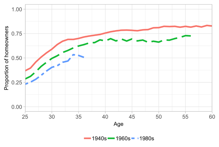
Southern Europe

Source: Own elaboration based on the Panel Study of Income Dynamics (PSID; top panel) and the Household Finance and Consumption Survey (HFCS; bottom panel). Southern Europe is a population-weighted average of Greece, Spain, Italy, Cyprus, Malta and Portugal. The graph represents the share of households that are living in owner-occupied housing, by age and decade of birth of the head of household (reference man for PSID data; reference person following the Canberra Group statistical criterion for the HFCS, which is usually the highest-earning member of a couple).
Role of changes in the labour market
Table 1
Relative contributions of different factors to changes in homeownership rates, age 30
1960s generation |
1980s generation |
|||
Labour market income dynamics |
68 |
73 |
||
Initial inequality |
61 |
41 |
||
Risk |
7 |
32 |
||
Asset returns and business cycle |
33 |
90 |
||
House price trend |
63 |
45 |
||
Cyclical factors |
-30 |
45 |
||
Borrowing conditions |
0 |
-68 |
||
Other factors |
-1 |
5 |
||
Note: This table summarizes the contribution of different factors to the drop in homeownership rates, according to model counterfactuals. The percentage values represent the share of the drop in homeownership rates (when comparing the 1960s and 1980s generations, respectively, to the 1940s generation) accounted for by one particular factor, taking into account its contribution to possible interaction effects. Negative values imply positive contributions to homeownership, and the right-hand column within each generation represents the breakdown of the components in the left-hand column.
Changes in earnings explain more than half of the decrease in homeownership rates (Table 1). For younger generations, career-long positions have become ever scarcer, unemployment spells are longer, and earnings inequality has increased (see Acemoglu and Autor, 2011; Goldin and Katz, 2009).[2] While the labour incomes of high earners have increased substantially over time in real terms, those on lower incomes have seen their real earnings stagnate or decrease. As a result, they find it harder to buy a home. Why? There are almost no homes on the market below a certain minimum price, quality or size threshold. Households too poor to access a mortgage for that minimum amount are thus shut out of the housing market.
According to the decomposition, earnings inequality accounts for 61% of the drop in homeownership rates for the 1960s generation. For those born in the 1980s, earnings volatility also plays an important role, explaining 32% of the drop at age 30. With less stable incomes, households are wary of making a large investment like buying a home and of assuming a large amount of gross debt. As a result, they stay renters for longer (Fisher and Gervais, 2011).
Favourable labour and housing markets at young ages are crucial
Over the past 60 years, the price of the median home has been gradually increasing relative to the median income. This evolution, which can be linked to cohort sizes, housing supply constraints, land-use policies, building regulations, housing characteristics, and other policies and institutions, was also a key reason for the reduction in homeownership.
The timing of fluctuations in house prices and the business cycle can leave a permanent mark on a generation. For instance, a generation that benefits from low house prices during its prime homebuying years is likely to be composed of more homeowners. And once households become homeowners, they tend to stay homeowners for most of their lives. Those born in the 1960s entered the housing market at a time when house prices were cyclically low, which helped counter other, negative forces impacting homeownership. For those born in the 1980s, the opposite was true, compounded by the effect of the 2008 crisis on their earnings.
Borrowing conditions have also fluctuated over time. In particular, loan-to-value (LTV) and loan-to-income (LTI) restrictions on mortgages were relaxed in the lead-up to the global financial crisis and became more stringent afterwards. The model suggests that easier borrowing conditions helped the 1980s generation get onto the housing ladder in the early 2000s.
This decomposition abstracts from general equilibrium effects of earnings dynamics and borrowing conditions on house prices. For instance, easier financing pushed up house prices during this period (Favara and Imbs, 2015), which would moderate its positive contribution to homeownership rates.
Implications for wealth accumulation
For most households, their primary residence is both the largest asset they hold and the majority of their wealth. Households buy houses to save, but also because they enjoy owning or to insure against rising future rents. Besides, homebuying is the only time most households incur substantial leverage, which implies their wealth can increase very rapidly if house prices rise.[3] As a result, a household that is left out of the housing market because of LTI or LTV restrictions might accumulate less wealth than it otherwise would, particularly at a time of low mortgage rates. This channel can reinforce the increase in wealth inequality derived from low real rates (Greenwald, Leombroni, Lustig, Van Nieuwerburgh, 2021).
Younger households are now more likely to participate in the stock market. However, these extra savings in the form of financial wealth do not seem to compensate for the missing housing wealth, as they are concentrated within richer households. In the United States, the median young household is less wealthy than a similar household was 20 years ago (Chart 2), and, because young households frequently hold little equity in their homes, these differences are likely to grow as they age.
Chart 2
Wealth accumulation by generation
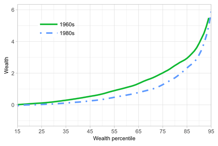
Note: The figure represents the average wealth accumulated by households in a given generation and position in the wealth distribution. Wealth is measured as multiples of average income in the economy at the time (US data, Survey of Consumer Finances).
Conclusions
The evolution of homeownership rates is closely intertwined with labour markets, housing markets and financial conditions. Thus, the design of labour market regulations, fiscal policies and the macroprudential framework should take into account their potential impact on young households trying to get on the housing ladder.
On the one hand, the 2000s boom-bust house price episode showed that there are risks for the financial system associated with highly levered homebuyers, and that building housing stock can divert resources from other productive sectors. On the other hand, a combination of policies that facilitates access to homeownership can help lower wealth inequality and increase social cohesion.
References
Acemoglu, D., and Autor, D. (2011), “Skills, tasks and technologies: Implications for employment and earnings”. Handbook of labor economics, Vol. 4, pp. 1043-1171, Elsevier.
Becker, S.O., Bentolilla, S., Fernandes, A. and Ichino, A. (2008), “Youth emancipation and perceived job insecurity of parents and children”, Journal of Population Economics, Vol 23, pp. 1047-1071.
Chetty, R., Sandor, L. and Szeidl, A. (2017), “The effect of housing on portfolio choice” Journal of Finance, Vol. 72, No 3, pp. 1171–1212.
Davis, S. J. and Haltiwanger, J. (2014), Labor market fluidity and economic performance No. w20479, National Bureau of Economic Research.
Favara, G. and Imbs, J., (2015), “Credit supply and the price of housing”, American Economic Review, Vol. 105(3), pp.958-92.
Fisher, J. D. and Gervais, M. (2011), “Why has home ownership fallen among the young?”, International Economic Review, Vol. 52, No 3, pp. 883-912.
Glaeser, E. L., Laibson, D. and Sacerdote, B. (2002), “An Economic Approach to Social Capital”, Economic Journal, Vol. 112, No 483, pp. 437-458.
Goldin, C. D. and Katz, L. F. (2009), The race between education and technology, Harvard University Press.
Greenwald D., Leombroni, M., Lustig, H and Van Nieuwerburgh, S. (2021), Financial and total wealth inequality with declining interest rates, Working paper.
Johnson, J.E. and Schulhofer-Wohl, S. (2019), “Changing patterns of geographical mobility and the labor market for young adults”, Journal of Labor Economics, Vol. 37(S1), pp. 199-241
Jordà, O., Knoll, K., Kuvshinov, D., Schularick, M. and Taylor, A.M. (2019), “The rate of return on everything, 1870-2015”, The Quarterly Journal of Economics, Vol. 134, No 3, pp. 1225-1298.
Laeven, L. and Popov. A. (2017), “Waking Up from the American Dream: On the Experience of Young Americans during the Housing Boom of the 2000s”, Journal of Money, Credit and Banking, Vol. 49, No 5, pp. 861-895.
Paz-Pardo, G. (2021), “Homeownership and portfolio choice over the generations”, Working Paper Series, No. 2522, ECB, February 2021.
Rohe, W. M., Van Zandt, S. and McCarthy, G. (2002), “Home ownership and access to opportunity”, Housing Studies, Vol. 17, No 1, pp. 51-61.
- The article was written by Gonzalo Paz-Pardo (Senior Economist, Directorate General Research, Monetary Policy Research Division). The author would like to thank Niccolò Battistini, Maarten Dossche, Michael Ehrmann, Alexander Popov and Zoë Sprokel for their comments, as well as Antilia Virginie for her assistance with the Household Finance and Consumption Survey (HFCS) data. The views expressed here are those of the author and do not necessarily represent the views of the European Central Bank and the Eurosystem.
- These developments have occurred jointly with what has been deemed as a reduction in the “fluidity” of the labor market (Davis and Haltiwanger, 2014): job finding rates, job losing rates, and job-to-job transition rates have declined over time. Furthermore, inter-state migration rates in the United States have decreased on average (Johnson and Schulhofer-Wohl, 2019).
- Historically, for many countries, the volatility-adjusted returns of housing, measured as Sharpe ratios, have been high and dominated those of stocks (Jordà, Knoll, Kuvshinov, Schularick, Taylor, 2019).