



House price booms and policy choices: insights from a meta-regression analysis
Published as part of the Financial Stability Review, May 2026.
This special feature examines policy-assignment dilemmas facing macroprudential authorities when housing markets boom: which instruments work best, on which objectives, and in combination with which other tools? It does so by revitalising Mundell’s Principle of Effective Market Classification,[1] the policy-space analogue of Ricardo’s comparative advantage principle, and by applying it to macroprudential policy. The analysis uses a novel G-search literature-search algorithm and an AI-supported, replicable data-extraction system to assemble estimates of policy-impact parameters from the empirical literature. It then distinguishes standard, instrument-by-instrument evidence, from jointly estimated policy-impact parameters, which are needed to account for rival instruments acting in the same empirical setting. Three findings emerge. First, the results confirm earlier meta-analytic evidence that macroprudential policy moderates household credit growth more clearly than it does house price growth, that tightening has more visible effects than loosening, and that instruments differ in their strengths and weaknesses. Second, joint estimates sharpen policy-assignment analysis by revealing how relative effects change when instruments are assessed together rather than alone. Third, applying the Mundell framework identifies instrument pairings that satisfy necessary conditions for substitutability or complementarity. Overall, the menu of options available to effectively tame housing market booms is wide, provided instruments are assigned to objectives by their relative – not absolute – effectiveness.
1 Introduction
The annals of financial-crisis history are replete with episodes of housing booms and busts. A familiar pattern recurs: house prices gradually rise, optimism strengthens, collateral values improve and borrowing increases. As the boom matures, rising housing wealth lifts consumption, easier credit conditions fuel further demand and confidence in continued price appreciation spreads through the economy. Yet these dynamics can leave the financial system increasingly fragile, as leverage rises, lending standards weaken and balance sheets become more exposed to the risk of price reversals. If a shock lands – whether tighter financing conditions, a reassessment of risk or a broader financial disturbance – the dynamic can reverse abruptly, typically at much greater speed than during the boom. Households cut spending, debt servicing problems emerge, losses spread to bank balance sheets and credit conditions tighten, leading to wider economic contraction. It is precisely to reduce the likelihood and cost of such episodes that macroprudential policy has developed as a domain in its own right, aiming to contain the build-up of housing-finance vulnerabilities before they become unmanageable. For central banks and other authorities, this raises a practical question: when housing markets boom, which policy tools are most effective in leaning against the build-up of vulnerabilities without imposing unnecessarily large costs on the broader economy?
The Tinbergen rule – prescribing one independent instrument for each independent objective – is a popular point of departure for answering policy-assignment questions. However, when instruments are not independent, the rule falls short.[2],[3] Before the global financial crisis, macroprudential toolkits were narrow in scope. Since then, they have expanded markedly to include capital-based measures, borrower-based tools and liquidity instruments. Furthermore, these instruments sit alongside broader housing-market policies which are themselves situated outside standard macroprudential policy toolkits – such as housing-related taxes and levies – that may affect credit and house prices.[4] In some jurisdictions, although not all instruments are macroprudential, there are now arguably more of them available than clearly defined objectives. Mundell’s Principle of Effective Market Classification (PEMC) can help in resolving the policy-assignment dilemma: instruments should be assigned to objectives according to their relative, not absolute, effectiveness. This is the same comparative-ratio logic that underpins the Ricardian principle of comparative advantage.[5] For macroprudential policy, this raises a demanding empirical question, because several authorities, each with their own responsibilities, may seek simultaneously to restrain housing credit growth and moderate house price inflation, while not always having a financial stability objective in mind. Existing meta-analyses have made useful progress on measuring average instrument effects, but they have not explicitly addressed this assignment question.[6]
This special feature examines these macroprudential policy-assignment questions through meta-regression analysis. Section 2 sets out the Mundell-Ricardo perspective for analysing policy-assignment issues and explains how meta-analysis can inform this conceptual framework through jointly estimated effects of policy actions on the growth of real household credit and real house prices. Section 3 describes the database-building approach that is applied to extract these policy-context conditional effects. Then, Section 4 reports unconditional findings on instrument effectiveness, while Section 5 turns to the jointly estimated effects and the assignment perspective. Section 6 concludes.
2 Many objectives and many tools: meta-analysis and the Mundell approach to policy-assignment
The starting point for assigning instruments is to treat Mundell’s PEMC as a general rule for policy-assignment. The question posed by Ricardo was: which country should produce which good? Mundell asked a different, yet similar – in the sense of the solution – question: which policy instrument should pursue which objective? In both cases, the answer depends on relative effectiveness rather than exclusivity. A country need not be absolutely the best at producing a good to possess a comparative advantage in it; likewise, a policy instrument need not be the most effective to be optimally assigned to a policy goal. Viewed this way, Mundell’s PEMC is the policy-space analogue of Ricardian comparative advantage.
The rise of macroprudential policy has, arguably, revived the relevance of Mundell’s PEMC. Before the global financial crisis (GFC), the binding constraint was Tinbergen’s: too few instruments for too many objectives. Today, the opposite problem can also arise. Macroprudential authorities frequently have several partially overlapping tools – capital-based instruments, sectoral risk weights, exposure limits, borrower-based limits, liquidity measures, etc. – all of which transmit through correlated channels to a smaller set of vulnerabilities. The risk is no longer one of too few instruments but, in some configurations, one of potentially overlapping instruments: redundancy, blurred accountability and over-assignment. Policy actions taken in housing market booms can illustrate the point. Housing market cycles have consequences not only for macroprudential policy but also for fiscal and social policies. If, for instance, a fiscal authority raises stamp duties to cool house prices for affordability reasons, the macroprudential authority is no longer operating in a closed policy space; another instrument has entered the same transmission channels.
The macroprudential meta-analytic literature has begun to establish an empirical basis for addressing policy-assignment issues. However, it has not yet posed the question directly. Four studies are particularly relevant. Araujo et al. provide the broadest synthesis, extracting more than 6,000 estimates from 58 studies and finding that tightening reduces credit growth more reliably than house prices, with borrower-based tools concentrating in the credit channel.[7] Kholodilin broadens the scope to include housing taxes alongside macroprudential regulations and, similarly, finds that both reduce loan growth and property prices.[8] Malovaná et al. focus on borrower-based instruments and find debt-service-to-income (DSTI) and debt-to-income (DTI) limits somewhat more potent on credit than loan-to-value (LTV) limits used alone;[9] a related capital-based meta-analysis finds that a 1 percentage point increase in capital requirements reduces annual credit growth by roughly 0.7 percentage points after correcting for so-called publication selection bias.[10][11] The qualitative message across these studies is fairly consistent: tightening has more visible countercyclical impacts on housing credit than on house prices, with marked heterogeneity across instruments.
What these studies share methodologically is also where a gap can be found. Each of them pools estimates of policy-impact parameters on an instrument-by-instrument basis, treating individual coefficients, not studies, as the unit of observation. None systematically addresses how the effectiveness of instruments compares when several are active at the same time, nor whether they substitute for or complement one another. These are assignment questions, and they require a different angle to be taken when analysing the evidence base: the subset of estimates produced from regressions in which more than one policy variable enters simultaneously. When two policy variables appear in the same empirical model, each estimated coefficient is interpreted as being conditional on the other policy variable and on the model’s other controls. The two estimates share the same outcome definition, sample, controls and identifying choices. When put on a common scale, through standardisation, they contain information about relative policy effectiveness within a common empirical environment. In other words, their comparative advantage, in the Mundellian sense, is revealed.
This special feature develops an approach to informing Mundell’s PEMC with meta-analysis findings in two complementary steps. Following a discussion in Section 3 of the approach taken to meta-database building, where coding for jointly estimated policy-impact parameters is key, it then reports the unconditional, instrument-by-instrument evidence (see Section 4), against which the prior meta-analyses can be benchmarked. It then turns to the jointly estimated subset (see Section 5), where the same exercise directly addresses relative effectiveness, overlap and trade-offs. The contribution is more organisational than it is econometric: by separating jointly estimated from individually estimated policy-impact parameters, the dataset can be queried to answer questions which the primary literature did not address explicitly. By zooming in on joint estimates, it sharpens the questions policymakers can ask of the evidence, shifting the discussion from “does this instrument work?” to “where is its comparative effectiveness greatest, and what is being missed when an instrument setting is calibrated in isolation?”
3 A novel approach to meta-database building
The conceptual framework for the discovery, screening and extraction pipeline for relevant policy-impact parameters is set out in Box A. This section describes its application to the present study, which is best viewed as an example of how an end-to-end pipeline can be deployed on an already-established meta-analysis literature. The four prior meta-analyses mentioned above provided a natural baseline of candidate studies for the studies analysed here. Still, because the meta-analysis question posed by each of these prior analyses was not the same as the one posed here, working from this baseline does not provide grounds for bypassing the discipline of a fresh systematic review: every candidate study was screened in precisely the same way.
The process moved through several stages, each building on the previous one. First, all primary studies cited in the four meta-analyses were retrieved, and those confirmed as containing extractable estimates while also meeting the target-variable/policy-variable pairing requirements for this study were retained.[12] Second, version snowballing – that is, searching for an earlier version of a published study – identified working-paper or pre-publication versions of journal articles; the rationale for retaining unique estimates from earlier versions is discussed in Box A.[13] Third, a version comparison index quantified the extent of unique content across model specifications, samples and reported estimates, with near-identical versions excluded to avoid double-counting. Throughout, the unit of inclusion is the estimate, not the study.
Terminology from the titles and keywords of the resulting baseline study set was used to calibrate the structured syntax of a smart bibliographic search. In this fourth step, the content words extracted from the titles and the author-supplied keywords of those studies were sorted by their marginal coverage of the calibration set, yielding an optimised search syntax. The syntax was then run against Web of Science and Scopus,[14] raising the candidate pool to 266 studies.[15] Fifth, already-discovered studies, verified as usable for the analysis, were removed to create a yet-to-be-screened short-list from this pool, and the remaining candidates were abstract-screened to retain only empirical studies of macroprudential policy effectiveness – excluding purely theoretical, DSGE and other simulation-based work. Sixth, the candidates were scored on a study relevance index (SRI), a data extraction complexity index (DECI) and a combined study usability score (SUS), reflecting the fit of the study to the dependent variables examined in this study and the manual effort required to convert findings into comparable quantitative evidence. Seventh, a final round of version snowballing was combined with backward snowballing (i.e. checking reference lists of eligible studies) with AI assistance to handle volume. 81 eligible studies emerged at the end of this data extraction process.
Box A
From search to synthesis: an end-to-end pipeline for metadata extraction
The credibility of any meta-analysis depends as much on how the evidence is assembled for a database as on how it is analysed. This box describes the metadata extraction pipeline used in the related special feature. It is designed to satisfy the Preferred Reporting Items for Systematic Reviews and Meta-Analyses (PRISMA) – the international reporting standard most top-tier journals expect of published systematic reviews. PRISMA requires that every stage of evidence assembly, from identification through screening to inclusion, is documented in a way that another researcher could reproduce. The pipeline described below was built around that requirement, using quantitative screening metrics. Rather than relying on the more usual qualitative approach to inclusion decisions,[16] each stage produces explicit numerical indices that can be audited end-to-end.
Smart search. Identification begins with a search strategy designed to recover known relevant studies efficiently while keeping the screening burden manageable. A “smart” meta-search, named G-search here, inverts the usual logic of query design. Rather than starting from a long, manually assembled list of candidate terms, it begins from calibration to a set of studies already known to be relevant and treats the content words in article titles and author-supplied keywords as data. The compact term set is then assembled using a greedy set-cover algorithm: at each step, the term that recovers the largest share of the calibration set not yet covered is added.[17] This produces short, auditable Boolean queries that are robust to the character-string limits imposed by some bibliographic platforms. The four-column structure in Table A.1 illustrates the result for the 63 calibration studies pooled from the four prior meta-analyses: synonyms of macroprudential policy, terms naming policy objectives, terms denoting effectiveness and terms identifying use of an empirical method. Two of the four columns recovered the full calibration set with seven or fewer terms; the remaining two came reasonably close.
Triage and structured extraction. Once a candidate study has been identified, the pipeline applies a structured triage and extraction process supported by an AI engine, used as a checking and extraction tool rather than a source of substantive judgement.[18] Each study receives three scores. A study relevance index (SRI) summarises how closely the paper matches the target dependent variables, policy instruments, their combinations, and other design features of interest. A data extraction complexity index (DECI) records the expected difficulty of converting the study into comparable quantitative evidence, given how completely the paper reports policy-impact parameter estimates, their precision metrics, samples and specifications. A study usability score (SUS), combining the previous two indices, sequences the coding effort while leaving the underlying scores visible for audit. Studies with sibling or earlier versions enter an additional version-control step, in which a version comparison index (VCI) assesses whether an earlier version contains unique estimates that the published version does not. Following recent best practice in the macroprudential meta-analytic literature, the unit of inclusion is the estimate, not the article: unique estimates from an earlier version are retained where they meet the same quality criteria; near-duplicates are excluded.
Layered metadata. Each retained estimate is stored within a layered metadata structure: Study → Analysis → Model → Estimate. This structure matters because a single empirical paper often contains several dependent variables, alternative specifications and many estimates, any subset of which may later prove relevant for moderator analysis or for the joint-estimation sub-sample analysis discussed in Section 5. Every estimate carries a hierarchical identifier, traceable back to its source, which makes errors easier to detect and corrections easier to propagate.
Replicability. The pipeline is designed so that two researchers working independently on the same topic, using the same inputs and settings, should be able to produce datasets that coincide closely. The combination of structured search, transparent scoring, version control and layered metadata ensures this: each decision is recorded, each filter is rule-based, and the role of the AI engine is confined to executing pre-specified instructions rather than exercising discretion. The pipeline therefore produces evidence that can be both audited and updated as new studies appear.
Limits. No automated pipeline removes the need for judgement. Calibration choices (e.g. choosing which prior meta-analyses to seed from), threshold settings on the SRI, DECI and SUS, and inclusion rules for version siblings all involve choices the researcher must justify. These are documented alongside the dataset rather than embedded in a “black box”. The aim is not to eliminate analyst judgement, but to make it visible.
Table A.1
The language of macroprudential policy effectiveness: construction of an efficient search string with the G-search algorithm
Four non-overlapping search strings for discovery of 63 studies on the effectiveness of macroprudential policy in taming housing market booms
(bibliographic search terms)
Boolean AND/OR | Macroprudential policy | AND Policy objective | AND Effectiveness | AND Empirical |
|---|---|---|---|---|
First term | Macroprudential policy (40) | Credit growth (21) | Effect (54) | Evidence (22) |
OR Second term | Macroprudential policies (11) | House prices (12) | Impact (6) | Banks (13) |
OR Third term | Loan-to-value ratio (4) | Household credit (8) | Affect (3) | Economies (8) |
OR Fourth term | Borrower-based measures (4) | Systemic risk (5) | Experience (2) | |
OR Fifth term | Macroprudential measures (2) | Housing market (4) | Credit register (2) | |
OR Sixth term | Macroprudential instruments (1) | House price growth (2) | Cholesky identification (2) | |
OR Seventh term | Macroprudential tool (1) | Financial stability (2) | Estimating (2) | |
OR Eighth term | Mortgage lending (2) | Causal forests (2) | ||
OR Ninth term | Housing loans (2) | Cointegration (1) | ||
OR Tenth term | Household leverage (1) | Household micro data (1) | ||
Total discovered | 63 | 59 | 63 | 55 |
Source: ECB calculations.
Notes: Each column in the table shows the incremental number of studies identified with the addition of one more term. Beyond the last populated row in each column, no term exists among the combined list of terms which can discover additional studies. If column search strings are combined, using the AND Boolean operator, the total number discoveries will equal the minimum shown in the “Total discovered” row. Lowered coverage, if applicable, must be traded-off against a potentially vast reduction in the number of studies to screen from a list produced by a curated database of peer-reviewed academic literature.
4 Unconditional findings: how potent are individual macroprudential policy instruments in taming housing market booms?
The unconditional evidence begins with the standard effectiveness question: do macroprudential instruments, on average and taken one at a time, slow the growth of real housing credit and real house prices? The metadata gathered for this special feature are broad enough to compare instruments but also narrow enough to preserve a common policy question. They focus on two target outcomes – the growth of real housing credit and real house prices – and on policy actions aimed at leaning against housing-cycle vulnerabilities. At the metadata-gathering stage, study relevance was scored in part according to whether instruments are core to macroprudential policy toolkits (capital-, borrower- and liquidity-based tools), peripheral (such as provisioning) or benchmark (such as housing taxes). The instruments differ in their point of contact with the housing market: borrower-based limits affect household borrowing capacity, lender-based measures affect bank incentives or balance sheet constraints, and housing-related taxes operate through the cost of buying or owning a home.
Chart C.1
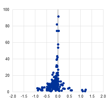
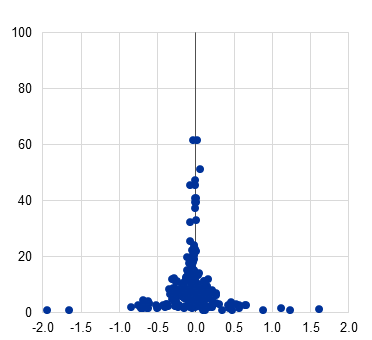
Evidence for countercyclical effectiveness of macroprudential policy is more dispersed for the growth of real household credit than real house price growth
a) Impacts on real housing credit growth | b) Impacts on real house price growth |
|---|---|
(x-axis: standardised effect (units of σ of the dependent variable), y-axis: precision (1/SE)) | (x-axis: standardised effect (units of σ of the dependent variable), y-axis: precision (1/SE)) |
 |  |
Source: ECB calculations, based on data extracted from academic studies.
Notes: Standardisation of effects is achieved by expressing them in units of standard deviations of the dependent variable (i.e. Y-standardisation). Precision is measured as the reciprocal of the standard error of the estimate, similarly Y-standardised. All estimates are included, covering capital-based, borrower-based, liquidity-based and housing-related tax measures. Where relevant, estimates are sign standardised (i.e. estimates for a loosening of macroprudential policy are re-expressed as “negative” loosening) for comparability.
Funnel plots provide an initial check on the distribution of extracted policy-impact parameter estimates before instrument-specific evidence is considered. Each point combines a standardised effect with a measure of its precision, facilitating the eyeballing of clustering, asymmetry and small-study effects (Chart C.1). These estimates measure the impact of activating macroprudential policies over the following four quarters. They are based on raw estimates, where -1/0/+1 indices were used in the primary studies to measure a loosening, a neutral stance or a tightening of policy tools. The evidence is more dispersed for housing credit than it is for house prices, with larger effects appearing more frequently for the former in the estimated impact distributions than they do for the latter. Also, several estimated impacts with high precision are situated close to zero or, in some cases, have an unconventional sign, thus calling for a deeper probe of the data for so-called publication selection bias.
Formal diagnostic testing can separate genuine effects from publication selection bias. If publication selection bias is absent from the data, the frequency distribution should be symmetric around the true effect. This is not the case for the two funnel plots shown in Chart C.1. The strength of asymmetry can be estimated using a funnel asymmetry test (FAT). Here, the FAT finds evidence of asymmetry for policy impacts on both the growth of real housing credit growth and of real house prices, pointing to publication bias which is stronger for household credit. A precision-weighted average (the PET column in Table C.1) is, therefore, very close to zero for both dependent variables. This is not because policies have no effect, but because publication selection bias is being averaged in with the signal. A precision-effect estimate with standard error (PEESE) can correct for this bias, with the corrected estimates markedly different from the uncorrected ones. Combining the impacts of all measures considered here, a macroprudential tightening reduces the growth of real housing credit by 0.037 and of real house prices by 0.022 standard deviations of the respective dependent variable over four quarters (Table C.1).
Table C.1
Correcting estimates of policy-impact parameters for publication selection bias
Summary statistics for all measures and all estimated effects
(cumulative four-quarter response to a macroprudential tightening, standardised)
Outcome variable | Sample size | Uncorrected effect | Evidence for publication selection bias | Bias-corrected effect |
|---|---|---|---|---|
Housing credit growth | 1,140 | -0.0005 | Very strong | -0.0369*** |
House price growth | 927 | -0.0098 | Strong | -0.0220*** |
Total observations | 2,067 |
Source: ECB estimates, based on data extracted from academic studies.
Notes: Standardisation of effects is achieved by expressing them in units of standard deviations of the dependent variable (i.e. Y-standardisation). They measure cumulative responses over four quarters to a tightening of a policy, expressed in units of standard deviations of the dependent variable. PET reports the intercept β₁ from the weighted regression effᵢ = β₀·SEᵢ + β₁ + εᵢ (weights = 1/SEᵢ²); under publication selection, β₁ is biased toward zero. PEESE reports β₁ from the analogous specification effᵢ = β₀·SEᵢ² + β₁ + εᵢ, which approximates more closely the non-linear relationship between an estimate and its standard error in the presence of selective reporting, yielding a less biased estimate of the underlying effect. The funnel asymmetry test (FAT) corresponds to the significance of β₀; its outcome is reported qualitatively in the fourth column, with “moderate”, “strong”, and “very strong” denoting rejection of the no-bias null at 10%, 5% and 1% significance. *** denotes statistical significance at the 1% level, ** the 5% level and * the 10% level.
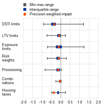
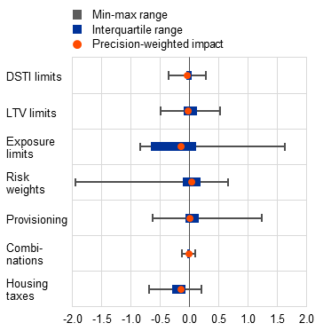
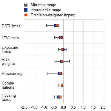
Instrument-level estimates suggest that the credit channel dominates the house price channel. Borrower-based instruments – especially DSTI but also LTV limits – appear to have material effects on credit. This is because they constrain households at the point where credit decisions are made, through either affordability or collateral limits (Chart C.2). Housing-related taxes stand out for a different reason: their reach extends visibly to both credit and house prices, consistent with their closer connection with the user cost of housing. By contrast, broad-based capital measures and some bank-balance-sheet tools show more muted or heterogeneous effects on housing credit. This is unsurprising. Broad-based measures are not specifically targeted at mortgage lending and may, depending on banks’ portfolio choices, allow credit reallocation across sectors rather than reducing mortgage credit directly. Their primary purpose is to strengthen borrower and lender resilience rather than to moderate the housing-credit cycle. Their main contribution to financial stability lies in that resilience role, which the unconditional credit-growth estimates do not capture.
Chart C.2
Macroprudential policy effectiveness appears to be stronger for real household credit growth than real house prices
a) Impacts on real housing credit growth | b) Impacts on real house price growth |
|---|---|
(standardised effects; ranges, precision-weighted impacts) | (standardised effects; ranges, precision-weighted impacts) |
 |  |
Source: ECB calculations, based on data extracted from academic studies.
Notes: Standardisation of effects is achieved by expressing them in units of standard deviations of the dependent variable (i.e. Y-standardisation). The combinations category groups instrument combinations which do not fit neatly under any one of the main macroprudential policy instrument categories: capital-based, borrower-based and liquidity-based tools. The charts depict the min-max and interquartile ranges, with precision-weighted impacts of each instrument on each dependent variable towards the centre. Precision-weighted impacts place greater weight on estimates with lower standard errors. Where relevant, estimates are sign standardised (i.e. estimates for a loosening of macroprudential policy are re-expressed as “negative” loosening) for comparability.
Particular caution is demanded in the interpretation of these averages. The precision-weighted summaries used here apply a conventional inverse-variance scheme commonly used in macroprudential meta-analysis. Precision is a statistical property: it captures how tightly an estimator pins down its target and it improves with sample size and reductions in residual variance. Identification quality is a separate property of the research design (i.e. whether the target is the right one). The two are conceptually distinct. A study can be highly precise about a biased quantity or imprecise about an unbiased one. Precision-weighting alone is therefore not a guarantee that the most credibly identified estimates receive the greatest weight. No consensus alternative weighting scheme exists, however, which is why inverse-variance weighting remains the standard summary device. Heterogeneity across study characteristics is addressed through moderator analysis, in line with the methodology literature.
Chart C.3
Macroprudential policy effectiveness in moderating real household credit growth appears to be stronger for tightening than for loosening
a) Impacts of tighter policy on real housing credit growth | b) Impacts of looser policy on real housing credit growth |
|---|---|
(standardised effects; ranges, precision-weighted impacts) | (standardised effects; ranges, precision-weighted impacts) |
 |  |
Source: ECB calculations, based on data extracted from academic studies.
Notes: Standardisation of effects is achieved by expressing them in units of standard deviations of the dependent variable (i.e. Y-standardisation). The combinations instrument category groups instrument combinations which do not fit neatly under any one of the main macroprudential policy instrument categories: capital-based, borrower-based and liquidity-based tools. The charts depict the min-max and interquartile ranges, with precision-weighted impacts of each instrument on each dependent variable towards the centre. Precision-weighted impacts place greater weight on estimates with lower standard errors. Where relevant, estimates are sign standardised (i.e. estimates for a loosening of macroprudential policy are re-expressed as “negative” loosening) for comparability.
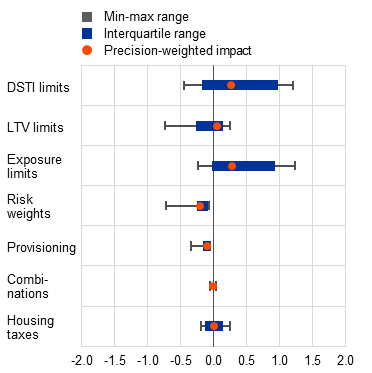
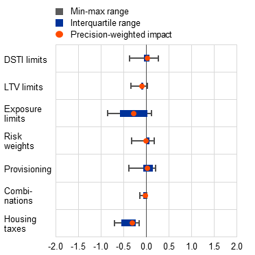
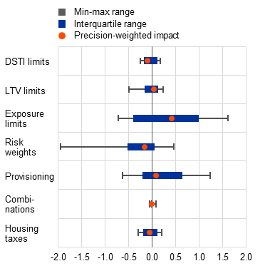
Visible asymmetries between the effects of tightening and loosening policy instruments reinforce a resilience-based interpretation of macroprudential policy effectiveness. Tighter measures are associated with clearer reductions in housing credit than looser measures are with increases (Chart C.3), and a similar but weaker pattern is found for impacts on real house prices (Chart C.4). This asymmetry should not be over-interpreted as evidence that loosening is impotent. Most underlying studies pool episodes unconditionally on the state of the financial cycle, while loosening is, by construction, deployed when credit is expected to contract – generating a selection bias that attenuates estimated effects. The relevant counterfactual is what credit would have done absent the action; reduced-form averages cannot distinguish “no effect” from “prevented a sharper contraction”. Better-identified bank- and loan-level evidence around actual releases, notably during the COVID-19 pandemic, finds that banks with greater capital headroom sustained lending more robustly. Releasable buffers also aim at preserving credit supply, not at stimulating demand. The absence of a positive credit impulse should, therefore, not be interpreted as evidence of policy impotence. The headline policy message to be drawn from these findings is consistent with the wider meta-analytic literature: tightening is often found to be more impactful on real household credit growth than on real house price growth. Also, borrower-based tools are found to have more meaningful effects on credit than other instruments. Notably, housing taxes appear to have a substantial impact on both credit and house prices. At the same time, the impacts of broader lender-based tools depend more on institutional structure, timing and bindingness. Overall, these findings are consistent with the view that the focus of macroprudential measures should unequivocally be on restraining the build-up of housing-finance vulnerabilities, rather than fine-tuning or lowering house prices.
Chart C.4
Macroprudential policy effectiveness in moderating real house price growth appears to be stronger for tightening than for loosening
a) Impacts of tighter policy on real house price growth | b) Impacts of looser policy on real house price growth |
|---|---|
(standardised effects; ranges, precision-weighted impacts) | (standardised effects; ranges, precision-weighted impacts) |
 |  |
Source: ECB calculations, based on data extracted from academic studies.
Notes: Standardisation of effects is achieved by expressing them in units of standard deviations of the dependent variable (i.e. Y-standardisation). The combinations instrument category groups instrument combinations which do not fit neatly under any one of the main macroprudential policy instrument categories: capital-based, borrower-based and liquidity-based tools. The charts depict the min-max and interquartile ranges, with precision-weighted impacts of each instrument on each dependent variable towards the centre. Precision-weighted impacts place greater weight on estimates with lower standard errors. Where relevant, all estimates are sign standardised (i.e. estimates for a loosening of macroprudential policy are re-expressed as “negative” loosening for comparability).
5 Conditional findings: how the marginal impacts of individual instruments can inform assignment
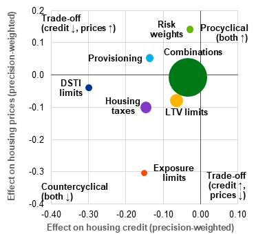
To move from effectiveness to policy-assignment, joint estimation of policy-impact parameters is key. When two or more policy variables enter the same empirical model, each coefficient is estimated conditional on the other policy variables and on the model’s remaining controls. The estimates therefore share an outcome definition, sample and identifying structure, making them closer to the policy environment in which authorities often act together rather than in isolation. This matters for an empirical application of Mundell’s principle because assignment depends on relative effectiveness: which instrument has the stronger impact on which objective? Chart C.5, panel a) shows a first mapping. Each instrument is located by its jointly estimated impact on real housing credit growth and real house price growth, using policy-impact parameters that are not yet corrected for publication-selection bias. The map is therefore a diagnostic starting point, not the final estimate of conditional effectiveness.
Chart C.5
Mapping policy impacts can reveal relative effectiveness and inform assignment
a) Standardised dual impacts of individual macroprudential policy instruments | b) Calibration of Mundellian assignment for LTV and DSTI limits to tame housing market booms |
|---|---|
(standardised effects; joint precision-weighted impacts) | |
 |  |
Source: ECB calculations, based on data extracted from academic studies.
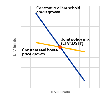
Notes: Panel a: standardisation of effects is achieved by expressing them in units of standard deviations of the dependent variable (i.e. Y-standardisation). The combinations instrument category groups instrument combinations which do not fit neatly under any one of the main macroprudential policy instrument categories: capital-based, borrower-based and liquidity-based tools. The chart depicts jointly estimated precision-weighted impacts of each instrument on real housing credit growth and real house price growth, and a measure of the precision of estimated impacts. Precision-weighting here is joint, but the measure used assumes independence. The metric places greater weight on estimates with lower standard errors around estimated impacts for both real housing credit growth and real house price growth. Where relevant, estimates are sign standardised (i.e. estimates for a loosening of macroprudential policy are re-expressed as “negative” loosening) for comparability. Panel b: each iso-target line is calibrated from the jointly estimated policy-impact parameters reported in Table C.3. With b1 denoting the joint coefficient on the y-axis instrument (here, LTV limits) and b2 the joint coefficient on the x-axis instrument (here, DSTI limits), the slope of the iso-target line in (DSTI, LTV) space is given by −b2 / b1. For the constant-credit-growth line, b1 = -0.0477 and b2 = -0.3182, giving a steep slope of approximately -6.67 − indicating that DSTI limits are relatively more effective on household credit. For the constant-house-price-growth line, b1 = -0.0695 and b2 = -0.0626, giving a much shallower slope of approximately -0.90 − indicating that LTV limits are relatively more effective on house prices.
For policy-assignment, the next step is to correct policy-impact parameters for publication selection bias. Table C.2 repeats the publication-selection-bias adjustment used earlier, but now only for jointly estimated policy impacts. The corrected impact on real housing credit growth is larger than in the full sample, with the PEESE estimate rising in absolute value from 0.0369 to 0.0661 standard deviations over four quarters. By contrast, the corresponding house-price estimate changes only modestly, from 0.0220 to 0.0251. This could mean that joint specifications isolate conditional effects more cleanly, but it could also reflect the narrower joint-estimate subset. The key diagnostic is whether instruments behave differently when estimated jointly rather than alone.
Table C.2
Correcting joint estimates of policy-impact parameters for publication selection bias
Summary statistics for all measures and jointly estimated effects
(cumulative four-quarter response to a macroprudential tightening, standardised)
Outcome variable | Sample size | Uncorrected effect | Evidence for publication selection bias | Bias-corrected effect |
|---|---|---|---|---|
Housing credit growth | 390 | -0.0265 | Very strong | -0.0661*** |
House price growth | 316 | -0.0095 | Moderate | -0.0251** |
Total observations | 706 |
Source: ECB estimates, based on data extracted from academic studies.
Notes: Standardisation of effects is achieved by expressing them in units of standard deviations of the dependent variable (i.e. Y-standardisation). PET reports the intercept β₁ from the weighted regression effᵢ = β₀·SEᵢ + β₁ + εᵢ (weights = 1/SEᵢ²); under publication selection, β₁ is biased toward zero. PEESE reports β₁ from the analogous specification effᵢ = β₀·SEᵢ² + β₁ + εᵢ, which approximates more closely the non-linear relationship between an estimate and its standard error in the presence of selective reporting, yielding a less biased estimate of the underlying effect. The funnel asymmetry test corresponds to the significance of β₀; its outcome is reported qualitatively, with “moderate”, “strong”, and “very strong” denoting rejection of the no-bias null at 10%, 5% and 1% significance. *** denotes statistical significance at the 1% level, ** the 5% level and * the 10% level.
For an interpretation of how joint estimates differ from the full sample of policy-impact parameters, a comparison of joint versus solo estimates provides the cleanest diagnostic. Solo estimates come from specifications in which one policy instrument is included; Joint estimates come from specifications in which two or more policy-impact parameters are estimated together (Table C.3). At the aggregate all-measures level, statistical tests find that differences are not significant, possibly reflecting PEESE non-linearities and instrument heterogeneity. Yet an instrument-level comparison is more revealing. For real housing credit growth, the joint impacts of LTV limits and risk weights are significantly smaller in absolute value than their solo impacts. For real house price growth, the joint impact of risk weights is significantly larger than the corresponding solo impact. When the aim is to assign instruments according to their relative effectiveness, even one such difference matters, because each instrument enters several pairwise slopes; mismeasuring one coefficient therefore propagates throughout the entire assignment map.
The assignment implications become more visible using Mundell’s original diagram. In Chart C.5, panel a, horizontal coordinates map the precision-weighted joint effects on real housing credit growth, while vertical coordinates map the corresponding effects on real house price growth, with bubble sizes scaled by joint precision.[19] The chart space can be divided into four regions: countercyclical, procyclical, and two trade-off regions where one objective falls while the other rises. Housing taxes sit firmly in the countercyclical region. DSTI limits look like a near-pure credit-moderating tool. LTV limits sit closer to housing taxes than to DSTI limits. Some lender-based measures, including risk weights and provisioning, fall into trade-off regions, indicating that their housing-cycle effects should be interpreted alongside their resilience role.
Table C.3
Comparing the information content of joint estimates of macroprudential policy-impact parameters with solo estimates
Solo and joint PEESE meta-regression estimates of macroprudential policy-impact parameters on the growth of real household credit and real house prices by instrument
(cumulative four-quarter response to a macroprudential tightening, standardised)
Impacts on real household credit growth | Impacts on real house price growth | |||||
|---|---|---|---|---|---|---|
Solo | Joint | Comparison | Solo | Joint | Comparison | |
All measures | -0.0922*** | -0.0661*** | Solo ≈ Joint | -0.0289*** | -0.0251** | Solo ≈ Joint |
DSTI limits | -0.3717*** | -0.3182*** | Solo ≈ Joint | -0.0441 | -0.0626 | Solo ≈ Joint |
LTV limits | -0.1395*** | -0.0477* | |Joint| < |Solo| | -0.0520* | -0.0695** | Solo ≈ Joint |
Exposure limits | -0.1688** | -0.2676* | Solo ≈ Joint | -0.1389 | -0.3669** | Solo ≈ Joint |
Risk weights | -0.0748*** | -0.0130 | |Joint| < |Solo| | 0.0238 | 0.2051** | |Joint| > |Solo| |
Provisioning | -0.1021*** | -0.1318*** | Solo ≈ Joint | -0.0281 | 0.0480 | Solo ≈ Joint |
Combinations | -0.0377*** | -0.0276** | Solo ≈ Joint | -0.0036 | -0.0019 | Solo ≈ Joint |
Housing taxes | -0.1347*** | -0.1669*** | Solo ≈ Joint | -0.0685** | -0.0598 | Solo ≈ Joint |
Source: ECB estimates, based on data extracted from academic studies.
Notes: Standardisation of effects is achieved by expressing them in units of standard deviations of the dependent variable (i.e. Y‑standardisation). In the columns headed Solo and Joint, *** denotes statistical significance at the 1% level, ** at the 5% level and * at the 10% level. Solo refers to PEESE meta-regression estimates derived from primary-study specifications in which a single macroprudential instrument is included; Joint refers to estimates derived from specifications in which two or more impact parameters are estimated jointly. The “Comparison” columns report the verdict of a one-sided directional z-test on the disjoint Solo and Joint sub-samples: cells flagged “|Joint| < |Solo|” or “|Joint| > |Solo|” indicate rejection at the 5% level, while cells reading “Solo ≈ Joint” indicate that the directional hypothesis cannot be rejected at that level. PEESE estimates follow Stanley, T.D. and Doucouliagos, H., “Meta-regression approximations to reduce publication selection bias”, Research Synthesis Methods, Vol. 5, Issue 1, March 2014, pp. 60-78.
From this mapping, a more explicit Mundell assignment exercise becomes feasible. Using the joint estimates in Table C.3, so-called iso-target lines can be drawn for combinations of two instruments that hold a target unchanged.[20] In the LTV-DSTI illustration (Chart C.5, panel b), the constant-credit-growth line is steep, because DSTI limits have a much larger relative effect on credit than LTV limits. The constant-house-price-growth line is flatter, because LTV limits are relatively more connected to house prices. The point is not that house prices should become the objective of macroprudential policy. The macroprudential objective remains the containment of housing-finance vulnerabilities and the resilience of borrowers and lenders. Rather, the diagram shows when an instrument’s strongest cyclical association differs from its usual institutional assignment.
The same framework can discipline the discussion of substitutability and complementarity of policy instruments. In the Mundell sense, two instruments are substitutes for a target when both push that target in the same direction, so that more of one can in principle offset less of the other along an iso-target line. They are complements when their coefficients have opposite signs, so that stabilising the target requires them to move in a coordinated way. This is a linear, conditional classification. It does not establish econometric complementarity in the cross-partial sense, because the primary-study specifications generally do not include interaction terms. The analysis therefore tests necessary conditions for Mundellian substitution or offsetting, not structural interaction effects.
Pairwise testing of policy instrument effectiveness can nevertheless add useful information beyond visual inspection. For each target and instrument pair, a procedure for testing individual effectiveness was carried out. It confirmed the joint sign configurations, computed relative-effectiveness slopes and their uncertainty, and tested whether implied substitution rates differed from one-for-one policy-impact parameters, with sensitivity to within-study correlation treated explicitly.[21] The findings are asymmetric across target variables. For real household credit growth, 15 of the 21 possible pairings are classifiable at the 10% level, six at the 5% level and three at the 1% level. DSTI limits feature prominently in policy instrument pairings for real household credit growth, while risk weights do not enter any classifiable pairing for this objective. For real house prices, only three pairings are classifiable, but all survive at the 1% level: LTV-Exposure limits as substitutes, and LTV-Risk weights and Exposure limits-Risk weights are classified as complements. Macroprudential policies which aim at moderating real household credit growth therefore have a wider menu of substitutable instruments to choose from, while house-price effects are sparser and more coordination-dependent.
These findings also reveal some policy-assignment dilemmas. For instance, housing taxes are outside the standard macroprudential toolkit and may be set for revenue, affordability or distributional reasons, yet they can materially affect the same targets that macroprudential authorities monitor. This can create a “right instrument in the wrong hands” issue: the instrument with the stronger cyclical impacts may be controlled by an authority pursuing different objectives, while the macroprudential authority may hold instruments that are second-best for the cyclical task but indispensable for resilience. The value of the Mundell perspective is therefore diagnostic. It helps authorities see where instruments overlap, where coordination may be needed, and where calibration needs to take account of actions taken elsewhere in the same system.
6 Concluding remarks
This special feature has examined what macroprudential policy can do when housing markets boom, how empirical evidence can be assembled more systematically, and how this can inform policy-assignment. It confirms earlier meta-analytic findings that macroprudential measures affect real household credit growth more visibly than they do real house price growth, that tightening effects are clearer than loosening effects, and that different instruments have distinct strengths and weaknesses. It does so by using a novel G-search literature-search algorithm, an AI-supported and replicable data-extraction pipeline, and a focus on jointly estimated policy-impact parameters. In that sense, the article offers a first practical application of Mundell’s Principle of Effective Market Classification to macroprudential policy-assignment.
Jointly estimated policy-impact parameters are needed for policy-assignment because authorities rarely activate instruments in isolation. When two or more instruments enter the same empirical model, their coefficients are conditional on one another, making them better suited to assessing relative effectiveness than estimates taken from separate specifications. This does not transform the framework into a mechanical rule for calibration. Rather, robust empirical measures of policy-impact parameters can serve as a complementary diagnostic tool, especially where an authority lacks the instrument that appears most effective and must consider a credible second-best.
The Mundell framework also makes the substitutability question multi-dimensional. Two instruments can be substitutes for one target but complements for another: for example, the LTV-risk weights pair cannot be classified with any degree of confidence as satisfying necessary conditions for either substitutability or complementarity in moderating real household credit growth, but they can be classified as complements for dampening real house price growth. The framework reaches its limits here, because it identifies necessary conditions from linear, jointly estimated coefficients rather than structural interaction effects. More primary studies with policy interaction terms would therefore help in showing when instruments truly reinforce one another, and future meta-analysis could extend the policy-assignment perspective to objectives beyond household credit and house prices.
Finally, the findings also point to practical dilemmas in overlapping policy spaces. Housing taxes, for instance, may materially affect variables monitored by macroprudential authorities even though they are fiscal instruments with broader objectives. Space constraints prevent a full display of all pairwise results, but the implication is clear: assignment, coordination and second-best choices deserve closer attention. Overall, the menu of options available to effectively tame housing market booms is wide, provided instruments are assigned to objectives by their relative – not absolute – effectiveness.
See Mundell, R.A. “The appropriate use of monetary and fiscal policy for internal and external stability”, IMF Staff Papers, Vol. 9, No 1, International Monetary Fund, 1962, pp. 70-79.
See Tinbergen, J., On the Theory of Economic Policy, North-Holland, Amsterdam, 1952.
Fahr, S. and Fell, J., “Macroprudential policy – closing the financial stability gap”, Journal of Financial Regulation and Compliance, Vol. 25, Issue 4, 2017, pp. 334-359.
See, among others, Araujo, J., Patnam, M., Popescu, A., Valencia, F. and Yao, W., “Effects of macroprudential policy: Evidence from over 6000 estimates”, Journal of Banking & Finance, Vol. 169, 107273, 2024, and Kholodilin, K.A. “The impact of governmental regulations on housing market: Findings of a meta-study of empirical literature”, Discussion Papers, No 2113, Deutsches Institut für Wirtschaftsforschung, 2025.
See Mundell, R.A., op. cit.
See Araujo, J. et al., op. cit.; Kholodilin, K.A., op. cit.; Malovaná, S., Hodula, M., Bajzík, J. and Gric, Z., “Bank capital, lending, and regulation: A meta-analysis”, Journal of Economic Surveys, Vol. 38, Issue 3, 2023, pp. 823-851; and Malovaná, S., Hodula, M., Gric, Z. and Bajzík, J., “Borrower-based macroprudential measures and credit growth: How biased is the existing literature?”, Journal of Economic Surveys, Vol. 39, Issue 1, 2025, pp. 66-102.
See Araujo, J. et al., op. cit.
See Kholodilin, K.A., op. cit.
See Malovaná, S. et al., Borrower-based macroprudential measures and credit growth: How biased is the existing literature?, op. cit.
See Malovaná, S. et al., Bank capital, lending, and regulation: A meta-analysis, op. cit.
Publication selection bias arises when studies producing statistically significant or “expected” results are more likely to be written up, accepted by academic journals and cited more frequently. In other words, what ends up in print may not always be a faithful record of all that was found by researchers, meaning that averaging reported estimates, which contain such bias, can be misleading.
Cross-checking that primary studies met requirements for this analysis was greatly facilitated by the meta-study set out in Araujo, J. et al., op. cit., as the authors make their underlying dataset publicly available.
For quality control, working papers or unpublished studies were only included if the related final version was published.
Web of Science and Scopus are large, curated databases of peer-reviewed academic literature that allow users to search publications across disciplines and track citations for research evaluation and policy analysis.
Total number of studies discovered by the search string displayed in Table A.1 as of 12 May 2026.
See Page, M.J. et al., “The PRISMA 2020 statement: an updated guideline for reporting systematic reviews”, BMJ, Vol. 372, n71, 2021.
See Chvátal, V., “A greedy heuristic for the set-covering problem”, Mathematics of Operations Research, Vol. 4, No 3, 1979, pp. 233-235, and Johnson, D.S., “Approximation algorithms for combinatorial problems”, Journal of Computer and System Sciences, Vol. 9, Issue 3, 1979, pp. 256-278. The greedy set cover algorithm was developed to handle problems where the objective is to “reach everything” using as few choices as possible, but where finding the perfect minimum is computationally too expensive. The greedy rule is straightforward: at each step, select the group that covers the largest number of items not yet covered, and repeat this step until everything is covered.
The prompt architecture used to structure and sequence AI interactions in this study was developed with the assistance of ChatGPT 5.5 Pro. Claude Opus 4.7 in adaptive mode was then used to implement this architecture for metadata collection. All research design decisions, inclusion/exclusion criteria and final interpretations are the author’s own. As such, the process conforms with the principles described in Cook, N. et al., “Guidance for the use of AI in the meta-analysis of Economics Research”, Journal of Economic Surveys, 2026.
Specifically, for instrument k, joint precision is measured as JPₖ = (SEₖ,credit² + SEₖ,price²)⁻¹, where SEₖ,credit and SEₖ,price denote the standard errors of the jointly estimated standardised impacts on real housing credit growth and real house price growth respectively. This metric gives greater visual weight to instruments whose estimated impacts are more precisely measured across both target variables, while abstracting from covariance between the two estimates.
To illustrate the point more rigorously, for a single target with coefficients β₁ on instrument X₁ and β₂ on instrument X₂ in the same model, the so-called iso-target line – that is, the locus of (X₁, X₂) pairs that holds the target constant – has a slope of −β₂/β₁. When β₁ and β₂ share the same sign, the slope is negative: more of one substitutes for less of the other, so the two instruments are substitutes. By contrast, when policy action requirements are offsetting, the slope is positive: more of one requires more of the other to hold the target constant, indicating complementarity. The slope of the iso-target line therefore reveals substitutability or complementarity without recourse to explicit interaction terms.
The testing procedure involved four steps. First, each coefficient was tested for individual statistical significance. Second, the joint sign configuration was tested using an intersection-union test, so that the substitutability or complementarity classification was not based on point-estimate signs alone. Third, the Mundell relative-effectiveness slope, −βⱼ/βᵢ, was computed with its standard error, allowing for the covariance between the two coefficient estimates where possible. Fourth, a linear-hypothesis test assessed whether the substitution rate differed from one-for-one. Within-study correlations used in the covariance term are estimated from jointly estimated within-study evidence, with sensitivity checks used where the relevant covariance is not directly reported.