
Energy prices and private consumption: what are the channels?
Published as part of the ECB Economic Bulletin, Issue 3/2022.
1 Introduction
The recent increase in energy prices raises the question of the extent to which households will reduce their consumption in response. With the global economy in the process of recovering from the coronavirus (COVID-19) pandemic, the prices of many commodities – including oil and gas – have soared over the last year or so. Since demand for energy is inelastic in the short run, those large price increases imply significant declines in households’ purchasing power, which will need to be absorbed through (i) reduced consumption of non-energy goods and services, (ii) a reduction in savings or (iii) an increase in income. This article assesses the extent to which those three margins are playing a role in the transmission of higher energy prices to aggregate consumption. In addition, it analyses the distributional impact of higher energy prices, as the effect on individual households tends to vary considerably. Since the distributional impact of such price rises has the potential to be very significant, that may warrant a separate policy response independently of the macroeconomic implications of those developments.
The rise in energy prices should be seen in the context of an exceptional economic recovery, but other factors are also playing a role. While the impact that energy prices have on consumption has been studied before, the recovery following the COVID-19 crisis is atypical from a historical perspective. Thus far, it has been characterised by a surge in global demand for durable and non-durable consumer goods, leading to unprecedented bottlenecks in production and trade, with households having accumulated record levels of savings in the course of the pandemic.[1] Moreover, the supply of energy has been hampered by a lag in the production of oil, as well as geopolitical tensions – especially Russia’s recent invasion of Ukraine – and technical disruptions affecting the provision of natural gas to European countries.[2] It is important to account for these confounding factors in order to understand the aggregate impact that higher energy prices will have on private consumption and formulate an appropriate policy response.
This article presents new evidence for the euro area and is structured as follows. Section 2 outlines relevant existing literature. Section 3 presents new empirical evidence from both an aggregate and a disaggregated perspective. The aggregate perspective focuses on identifying the source of energy price fluctuation, while the disaggregated perspective focuses on distributional implications beyond the aggregate impact. Importantly, in order to provide a timely assessment of the macroeconomic and distributional implications of large changes in energy prices, the aggregate and disaggregated analyses are both based on survey data. Section 4 concludes and identifies a number of policy implications.
2 Existing literature
When countries are net importers of energy, higher energy prices generally entail a worsening of their terms of trade. Backus and Crucini showed, using a set of industrialised countries, that a large percentage of the variability of terms of trade is associated with extreme movements in oil prices.[3] They studied the terms of trade and their correlation with other variables in a setting in which events affecting the production of oil interacted with the production and sale of other goods. De Michelis et al. found that oil price increases generally drive a wedge between consumption developments in oil-importing and oil-exporting countries.[4] Higher oil prices transfer wealth from oil importers to oil exporters, and that wealth effect, in turn, has a negative impact on consumption in oil-importing countries through multiplier effects. It is worth noting that this impact may be larger in sectors which produce goods that are complementary to the consumption of oil, such as the automobile sector.
Higher energy prices do not always lead to a contraction in consumption; indeed, they can also be a consequence of increased consumption. Kilian, for example, showed that changes in the price of oil can reflect both oil supply shocks and shocks to global demand.[5] The economic impact of an oil price change which is caused by an unanticipated aggregate global demand shock will be very different from that of an oil price rise which is caused by an unanticipated shortfall in the production of oil. Hence, it is important to understand the extent to which increases in the price of oil are driven by different kinds of shock before formulating policy responses. Bodenstein et al. argued that the source of an oil shock matters greatly for the optimal monetary policy response to fluctuations in energy prices.[6] They looked at a wide range of monetary policy rules and identified an easily implementable welfare-maximising rule whereby the central bank puts zero weight on the price of oil, but responds to wage inflation. In the wake of fluctuations in oil prices, stabilising wage inflation fosters the stabilisation of core inflation, in line with earlier findings by Aoki.[7] When oil prices rise as a result of an increase in aggregate demand, wages also rise, and monetary policy will need to become tighter. Conversely, if oil prices increase as a result of disruptions in oil supply, and there are no second-round effects on wages, monetary policy does not need to tighten in order to stabilise core inflation.
Large increases in energy prices can affect individual households in very different ways. For example, Michael and Hagemann showed that exposure to higher energy inflation differs widely across individual households in the United States.[8] Because they spend a relatively large percentage of their income on energy, poor households are particularly hard hit in terms of inflation when energy prices surge. Hobijn and Lagakos confirmed those earlier findings, but also found that households which face higher than average inflation in one year (owing to higher energy prices) are not very likely to be confronted with the same inflation disparity the following year.[9] This implies that poorer households do not, over time, systematically face higher inflation as a result of their higher relative expenditure on energy. At the same time, it suggests that, in the case of a large energy price shock, the adverse impact on some households may be so large that it easily outweighs any positive impact seen through macroeconomic channels (e.g. employment).
3 Empirical evidence from the euro area
Aggregate perspective
Energy prices affect private consumption through both direct and indirect channels. An increase in energy prices directly affects households’ purchasing power through higher prices for energy products (electricity, gas, petrol, heating oil, etc.). In the euro area, about 30% of all energy use takes the form of final consumption – i.e. the use of such products by consumers (Chart 1). The remainder involves energy being used in the production of non-energy goods and services (i.e. intermediate consumption). A rise in energy prices entails an increase in the production costs of non‑energy sectors and – to the extent that producers of non‑energy goods and services adjust their final prices – a further direct reduction in households’ purchasing power. If those costs cannot be passed on to the final prices of the relevant goods, there will be an indirect impact on households’ purchasing power, since producers in the relevant sectors will either cut wages or have lower profits to distribute. Moreover, in advanced economies that are large producers of energy (e.g. Canada, Norway, the United Kingdom and the United States), indirect effects through the wages and profits of energy producers are also important.
Chart 1
Energy use and prices in the euro area
(left-hand scale: EUR billions; right-hand scale: index, 2015=100)

Sources: Eurostat and ECB calculations.
Notes: “Energy” refers to the sum of coke, refined petroleum products, electricity, gas, steam and air conditioning. Data are based on basic prices. The “real energy price” indicates the ratio of the energy component of the HICP to the overall index.
The impact of energy price changes on real disposable income can be proxied by the ratio of the GDP deflator to the private consumption deflator. For net importers of energy (such as the euro area), energy prices exhibit a stable negative correlation with the terms of trade, interpreted as the amount of imported goods that an economy can purchase per unit of exported goods. When assessing the impact that energy price changes have on consumption, a key proxy is the ratio of the GDP deflator to the private consumption deflator (or that of the income deflator to the spending deflator).[10] In the euro area, (real) energy prices are negatively correlated with that ratio (Chart 2). That measure is well‑founded from a theoretical perspective and captures both direct and indirect channels through which energy prices affect households’ real disposable income.[11] Even if the channels through which energy prices affect the economy change, this approach still shows stability in the relationship between energy-induced changes in purchasing power and private consumption. This is relevant in the face of changes to the energy intensity of consumption and innovations in the production of energy and non-energy goods.
Chart 2
Energy prices and the terms of trade
(index, 2010 average=100)

Sources: Eurostat, European Commission and ECB calculations.
Notes: The “real energy price” indicates the ratio of the energy component of the HICP to the overall index. “Terms of trade” are computed as the GDP deflator divided by the private consumption deflator. Owing to limited availability, data before 1995 are drawn from the Eurosystem macroeconomic projections database.
Well-known episodes involving large swings in energy prices highlight the role of different transmission channels. Chart 3 breaks the dynamics of households’ real disposable income down into various sources of income derived from economic activity (wages, profits and other property income), net transfers from the government, and the terms of trade (proxied by the ratio of the GDP deflator to the private consumption deflator). Fluctuations in the terms of trade stemming from large changes in the supply of energy appear to have been an important driver of household income after (i) OPEC increased oil production, leading to a collapse in energy prices in the first quarter of 1986, and (ii) Iraq invaded Kuwait, leading to soaring energy prices in the third quarter of 1990. In contrast, developments in aggregate economic activity appear to have been the main channel for the drop in household income in the fourth quarter of 2008 following Lehman Brothers’ default, amid falling energy prices and ensuing gains in the terms of trade. In the early stages of the COVID-19 pandemic, the abrupt fluctuations in economic activity were the main transmission mechanism, whereas the terms of trade weighed on household income at the end of 2021. However, in order to identify the underlying drivers, we need to use indicators with greater timeliness and frequency, such as survey data.
Chart 3
Households’ real disposable income and consumption
(annual percentage changes and percentage point contributions)
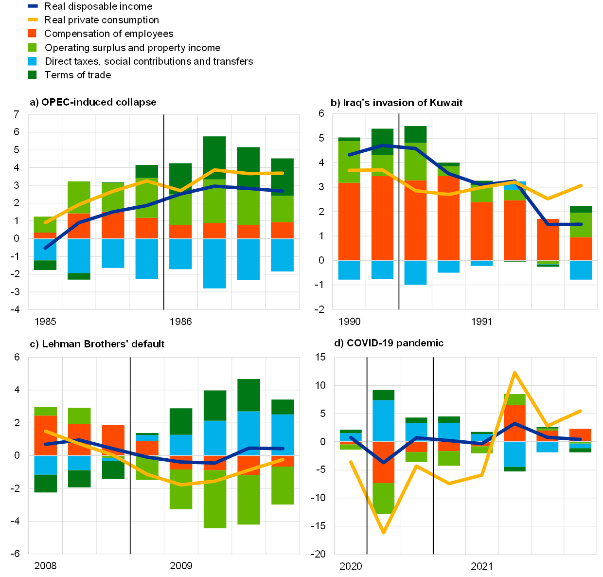
Sources: Eurostat, Eurosystem, European Commission and ECB calculations.
Notes: In the first three panels, the vertical line indicates the start of the episode in question. In panel d, the first vertical line denotes the beginning of the pandemic and the second line indicates the start of the rise in energy prices. Owing to limited availability, data for episodes before 1995 and for the fourth quarter of 2021 are drawn from the Eurosystem macroeconomic projections database.
Household surveys provide timely and frequent information on inflation and private consumption, as well as their underlying drivers. Historically, the index indicating households’ plans to make major purchases in the next 12 months that is derived from the European Commission’s consumer survey has tracked year‑on‑year growth in real private consumption of durable goods reasonably well, although the correlation between the two declined substantially during the first wave of the pandemic (Chart 4). Moreover, that survey-based indicator of households’ consumption expectations exhibits good leading properties with regard to actual future consumption.[12] Indeed, surveys contain information that may help with the timely identification of underlying drivers of households’ consumption decisions (Box 1). Increases in expected inflation can be driven by various factors, and some factors can potentially have opposite effects to others in terms of households’ spending plans. In the context of strengthening economic activity with higher levels of “demand-pull” inflation, consumption may rise as real income increases. However, in the presence of weakening economic activity with higher levels of “cost-push” inflation, consumption may fall instead as real income declines.
Chart 4
Fluctuations in consumption over time
(left-hand scale: standardised index, long-run average=0; right-hand scale: annual percentage changes)

Sources: Eurostat, European Commission and ECB calculations.
Notes: “Expected expenditure on major purchases” represents quarterly averages for a standardised index based on consumers’ net responses to questions about plans to make major purchases in the next 12 months. For the period up to (and including) 1989, data on “real private consumption of durables” relate only to France, with Finland being added to the series in 1990 and Germany being added in 1991; as of 1995, the data represent euro area aggregates. The vertical lines denote the first quarter of 1986 (OPEC-induced collapse), the third quarter of 1990 (Iraq’s invasion of Kuwait) and the fourth quarter of 2008 (aftermath of Lehman Brothers’ default).
Thus far, the recovery in consumption has been driven primarily by demand tailwinds, but cost-push headwinds are increasingly clouding the near-term outlook. In the early stages of the pandemic, as their financial prospects deteriorated, households scaled back their consumption and saving plans, mainly in response to contractionary cost-push shocks and, soon afterwards, demand-pull shocks (Chart 5).[13] Since early 2021, strong demand-pull shocks have contributed to recoveries in households’ expected financial conditions, consumption and savings. However, the rise in commodity prices that has been observed since the summer of 2021 has increasingly been regarded as stifling households’ expected financial situation, thus weighing on their spending plans. In March 2022, supply‑side contractionary forces – exacerbated by the ongoing geopolitical tensions – more than offset demand-side expansionary factors driving consumption plans.
Chart 5
Demand-pull and cost-push drivers of the expected consumption, financial situation and savings of households
(contributions to standard deviations from long-term averages)
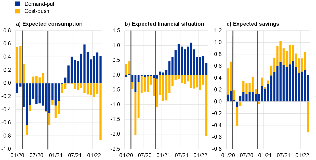
Sources: European Commission and ECB calculations.
Notes: For details of the estimation process, see Box 1. In each panel, the first vertical line indicates the beginning of the COVID-19 pandemic and the second denotes the start of the rise in energy prices.
Box 1
Disentangling demand-pull and cost-push forces: does it matter for consumption?
This box uses an empirical time series model to assess the role that households’ perceptions of the economy play in determining their plans to make major purchases. The European Commission’s consumer survey measures households’ expectations about economic activity and inflation, as well as their own spending plans, financial situation and savings. A structural multivariate (vector autoregression) model has been estimated using survey data for the period from January 1985 to February 2022. In order to disentangle the various structural drivers, the model assumes that expected economic activity improves after a perceived demand-pull shock and declines after a cost‑push shock, while both shocks lead to higher inflation expectations. The goal of this box is to look at the ways in which households’ expected consumption, financial situation and savings react to such shocks. Consequently, the responses of those three variables are left unrestricted.[14]
The responses to demand-pull and cost-push shocks suggest that the sources of such shocks matter for households’ expected consumption, financial situation and savings (Chart A). In order to compare the magnitude of the responses to the various shocks, each shock is standardised so as to entail the same impact (i.e. 1 standard deviation) on expected inflation. Hence, the standardised demand-pull and cost-push shocks induce observationally equivalent inflation pressures, but their economic impact is strongly asymmetrical. In line with theoretical predictions, households’ expected consumption, financial situation and savings improve significantly after a perceived demand-pull shock and deteriorate after a perceived cost-push shock. Moreover, confirming typical identifying assumptions in empirical literature, the results show that cost-push shocks have a more persistent impact on households’ expected consumption, financial situation and savings over the following two years relative to demand-pull shocks. Finally, looking at the horizon as a whole, households’ expectations appear to react more strongly to cost-push shocks than demand-pull shocks.[15]
Chart A
Responses to demand-pull and cost-push shocks
(x-axis: months; y-axis: standard deviations)

Sources: European Commission and ECB calculations.
Notes: This chart reports responses to standardised demand-pull and cost-push shocks entailing a 1 standard deviation impact on expected inflation. The solid lines indicate the median response, while the dotted lines indicate the upper and lower bounds of 68% credibility bands.
Analysis of the drivers of household inflation expectations around the time of well-known historical episodes validates the choice of identifying assumptions (Chart B). For instance, the model is good at capturing the cost-push nature of the decline in expected inflation that resulted from the increase in OPEC oil production and the ensuing collapse in oil prices in the first few months of 1986. Cost‑push forces also explain most of the surge in consumer price expectations that was triggered by the bout of oil price inflation which followed Iraq’s invasion of Kuwait in the summer of 1990. Moreover, the model correctly depicts the demand-driven drop in expected inflation following Lehman Brothers’ default in the second half of 2008 at the start of the global financial crisis. Overall, the model appears to accurately depict changes in consumer price expectations in response to both demand‑pull and cost-push forces.
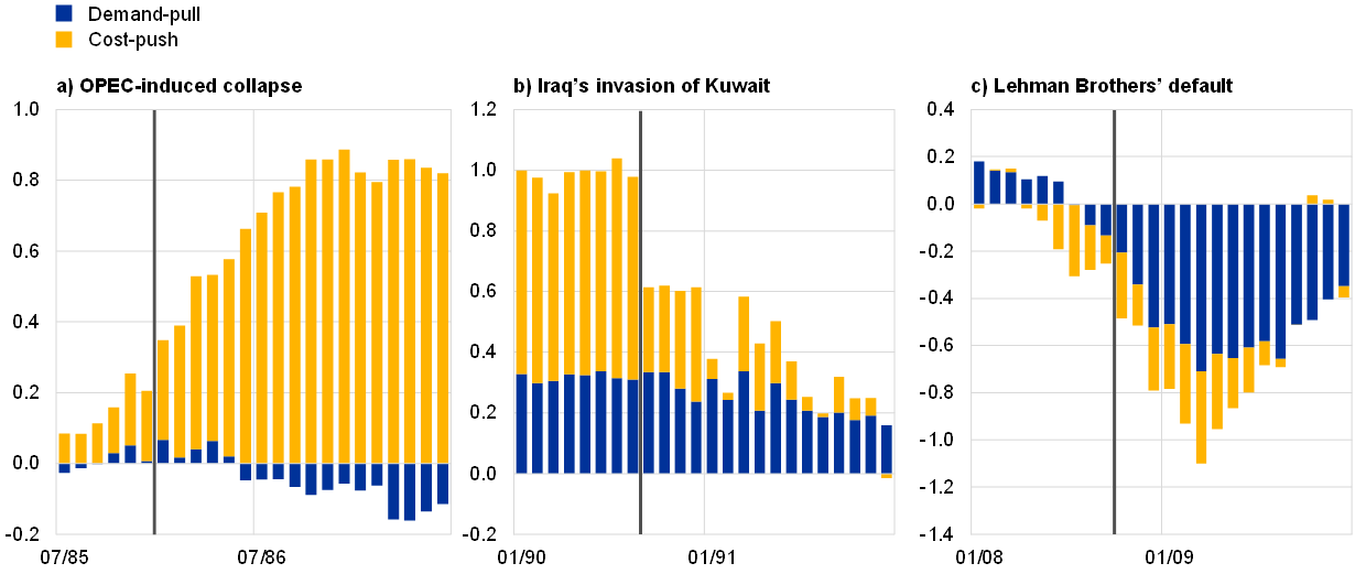
Chart B
Contributions of demand-pull and cost-push forces during key episodes
(left-hand scale: contributions to standard deviations from long-term averages; right-hand scale: annual percentage changes)
Expected inflation
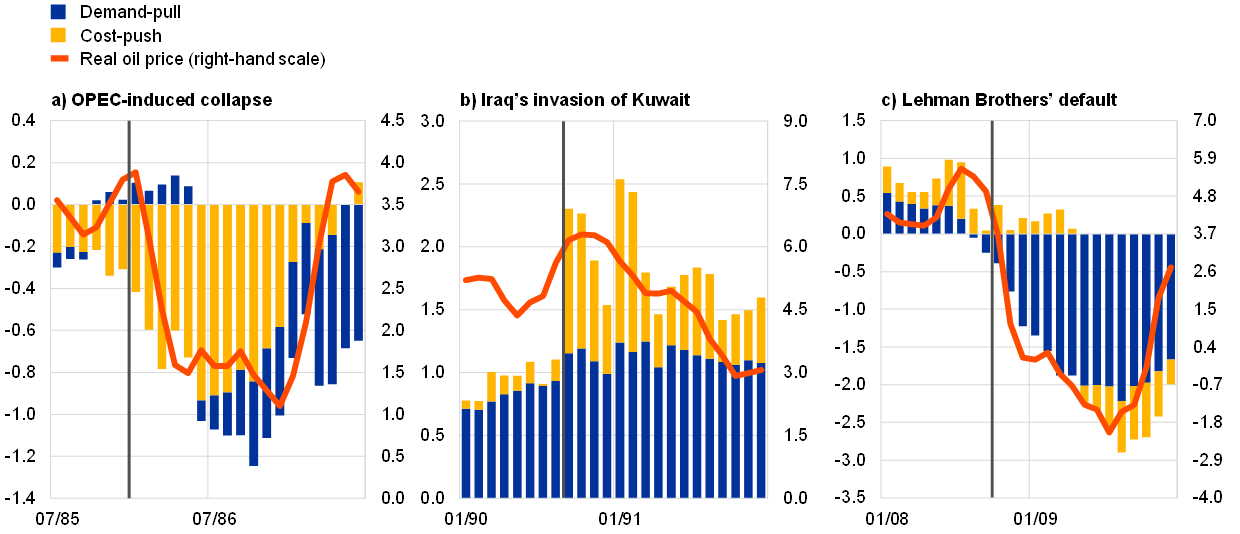
Expected consumption
Sources: European Commission, US Energy Information Administration, US Bureau of Labor Statistics and ECB calculations.
Note: The “real oil price” is calculated as refiners’ acquisition costs for (imported) crude oil divided by the consumer price index.
Looking at expected consumption during those same episodes, cost-push forces led households to step up their consumption plans during the OPEC-induced collapse in the first few months of 1986 and abruptly downsize them in the wake of Iraq’s invasion of Kuwait in the summer of 1990. In contrast, following Lehman Brothers’ default in the second half of 2008, the persistent downward pressure that was exerted on expected consumption stemmed mainly from demand-pull forces. Overall, cost-push forces appear to be the main drivers in episodes originating from the energy sector (especially the oil market).
Disaggregated perspective
While a change in energy prices can have several origins, an individual household will tend to perceive it as an exogenous shock to its real disposable income. When making decisions on consumption and savings, households take energy prices as a given, not considering the implications that their decisions have for energy prices. When energy prices rise, it leads to a reduction in households’ real disposable income, even if that price rise is caused by increased demand for energy. Depending on the aggregate economic conditions, a rise in energy prices will either exacerbate any decline in disposable income or partly offset any increase (e.g. in the context of an economic upturn). For those reasons, this section focuses on the direct distributional effects of changes in energy prices, while controlling for the underlying macroeconomic drivers of energy shocks, which were explored above in the section on the aggregate perspective.
Energy is a necessary consumer good, so household exposure to fluctuating energy prices declines as income rises. Since energy consumption responds to basic needs, which households cannot give up entirely, demand for energy tends to be price inelastic in the short run. Households typically accommodate any rise in energy prices by revising their saving plans and reallocating spending. However, the extent to which households need to resort to either of those strategies depends on their exposure to energy repricing. The share of households’ monthly income that goes on utilities and transport services (i.e. energy-intensive consumption) is an approximate indicator of their exposure to an energy price change. That exposure differs widely across income groups, standing at almost 35% for the lowest quintile of the income distribution but less than 10% for the top quintile.[16] Thus, the distributional effects of a rise in energy prices are sizeable, with low-income households facing almost four times the impact that is experienced by households in the top quintile of the income distribution (Chart 6).[17]
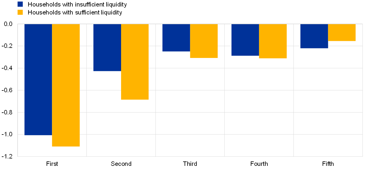
When spending on energy rises, households reduce their purchases of essential goods and services to a small extent. The average elasticity of substitution between spending on energy and other essentials (e.g. groceries, housing and health services) is fairly low, albeit the response varies across income quintiles (Chart 7; see Box 2 for details of the estimation methodology). Where basic needs are met primarily through low-cost items (which is the case for the households with the lowest incomes), there is very limited scope to compress spending on other essentials in response to rising energy prices (with that scope estimated at 0.2 percentage points of total spending for each percentage point rise in energy spending).[18]
Chart 6
The exposure of households to energy price shocks
(x-axis: income quintiles; y-axis: percentages)

Sources: Consumer Expectations Survey and ECB calculations.
Note: Figures are based on CES results for January 2022 and represent weighted averages of data for Germany, France, Italy, Spain, the Netherlands and Belgium.
Higher-income households make fewer adjustments to their spending on essentials, as energy-sensitive spending accounts for a smaller percentage of their income. For the same absolute increase in energy spending, households in the top quintile of the income distribution reduce their spending on essentials by just 0.15 percentage points. Middle-income households tend to react more, being more likely to replace branded products with lower-cost alternatives.[19] Within income quintiles, liquidity‑constrained households (i.e. those whose net income is insufficient to cover total spending and debt repayments) tend to cut their consumption of essentials somewhat more than those that have a liquidity buffer for unexpected expenses.
Chart 7
Changes in spending on essentials when energy spending rises
(x-axis: income quintiles; y-axis: percentage points of total monthly spending)

Sources: Consumer Expectations Survey and ECB calculations.
Notes: The vertical axis shows the average reduction in spending on essentials in response to a rise in energy spending. For each income quintile, energy spending rises by an amount equivalent to a 1 percentage point increase in energy’s share of the average income of the first quintile of the distribution. The equation in Box 2 estimates the percentage point change in the share of total spending on essentials that results from a 1 percentage point increase in utilities’ share of income. To obtain the average response to the same absolute change in spending on utilities, the beta coefficients are adjusted using the ratio of the average income of each quintile to the average income of the first quintile. The blue bars show the average responses of households without positive saving flows; the yellow bars show the average responses of households with positive saving flows. Estimates have been computed using a sample spanning the period from April 2020 to January 2022.
Chart 8
Changes in savings in response to a rise in energy spending
(x-axis: income quintiles; y-axis: percentage points of income)
Sources: Consumer Expectations Survey and ECB calculations.
Notes: The vertical axis indicates changes in households’ saving ratios in response to a rise in spending on utilities. For each income quintile, spending on utilities rises by an amount equivalent to a 1 percentage point increase in utilities’ share of the average income of the first quintile. The chart distinguishes between the responses of households with a liquidity buffer (yellow bars) and those without (blue bars). Estimates have been computed using a sample spanning the period from April 2020 to January 2022.
Households draw on their savings to cushion the impact that higher energy prices have on consumption. Empirical evidence confirms that – in the short run, at least – households substantially reduce their saving ratios in order to accommodate increased spending on energy (albeit to a lesser extent if liquidity buffers for unexpected expenditure are limited).[20] Identifying the responses of savings across different income quintiles reveals that, for the same absolute increase in energy spending, the reduction in savings is inversely correlated with the family’s income and about five or six times greater for households in the lowest quintile of the income distribution relative to those in the top quintile (Chart 8).
Box 2
Estimating household responses to changes in energy spending
This box presents details of the econometric methodology which has been used to study the effect that changes in monthly energy spending have on households’ saving ratios and spending on essentials. That analysis, which uses microdata from the ECB’s Consumer Expectations Survey, covers the six largest economies in the euro area, with more than 75,000 observations over the period since April 2020. Each quarter, the CES collects information about households’ monthly spending in 12 major areas (including utilities, transport services, food, health and housing services). Saving flows are derived by subtracting total monthly spending from monthly net income. “Essential” spending refers to food, beverages and tobacco, health and housing services.
Two linear panel models looking at quarterly changes in the monthly saving ratio and spending on essentials as a share of total spending are specified as a function of the quarterly change in the percentage of income that is spent on utilities (:

That equation includes the monthly saving ratio of three months earlier which captures the impact of major one-off purchases in the previous period that have repercussions for the saving ratio.
This analysis faces a number of challenges. Households may find it difficult to accurately recall all of their spending, broken down by category, so they may potentially misreport their total spending. The use of first differences in the specification partly controls for these issues, eliminating any household-specific constant biases in the data. The specification also includes several fixed effects with the aim of identifying the key parameter β, which measures the reaction to a change in spending on utilities, controlling for several confounding effects. Those fixed effects relate to (i) households’ heterogeneous characteristics (αj), such as the size and location of inhabited dwellings, and the composition of families, (ii) country-specific but time-varying factors (αc,t), such as the differing economic conditions that characterise individual countries (GDP growth, inflation rates, etc.), and (iii) factors that vary across income groups and over time (αi,t) which can influence decisions on savings and spending, such as government measures mitigating the pandemic’s impact on households.
Households with greater exposure to energy prices view measures aimed at easing the burden of rising energy prices as less adequate. Government intervention is primarily aimed at mitigating the unequal impact that rising energy prices have across households, supporting poorer households (who tend to spend more on energy as a share of their income). Despite benefiting most from them, households with very high exposure to energy prices tend to take the view that those policies are not sufficient to compensate for the negative impact of energy price spikes (Chart 9).
Chart 9
Perceived adequacy of government interventions and energy exposure
(x-axis: spending on utilities as a percentage of total income; y-axis: perceived adequacy of intervention on a scale of 0 to 10)

Sources: Consumer Expectations Survey and ECB calculations.
Notes: The vertical axis indicates the average score given by households to government measures aimed at curbing the impact that rising energy prices have on disposable income. Households in Germany, France, Italy, Spain, the Netherlands and Belgium are grouped together in 11 equally sized bins on the basis of their spending on utilities as a percentage of total income. For each bin, average spending on utilities as a percentage of total income is plotted against the corresponding average for the perceived adequacy of government measures. These data were collected in October 2021.
4 Conclusions
The recent rise in energy prices is a clear headwind for the recovery in consumption. In the early stages of the pandemic, as their financial prospects deteriorated, households scaled back their consumption plans, mainly in response to contractionary cost-push shocks and, soon afterwards, a series of negative demand‑pull shocks. Since early 2021, positive demand shocks have led to a recovery in households’ expected financial conditions, consumption and savings. However, the rise in commodity prices that has been observed since the summer of 2021 has increasingly been regarded as stifling households’ expected financial situation, thus weighing on their spending plans.
Increases in energy prices have significant distributional implications, which call for targeted fiscal policy measures. The impact that energy prices have on household income and spending depends primarily on the household’s level of exposure. Low‑income households with high levels of exposure tend to experience considerable financial distress when energy spending rises unexpectedly, and they respond to such shocks by reducing savings or delaying payments. As a result, those households are more likely to feel that there is a need for governments to mitigate the adverse impact of higher energy prices.
See the box entitled “Sources of supply chain disruptions and their impact on euro area manufacturing”, Economic Bulletin, Issue 8, ECB, 2021, and the box entitled “COVID-19 and the increase in household savings: an update”, Economic Bulletin, Issue 5, ECB, 2021.
See the box entitled “Natural gas dependence and risks to euro area activity”, Economic Bulletin, Issue 1, ECB, 2022.
Backus, D. and Crucini, M., “Oil prices and the terms of trade”, Journal of International Economics, Vol. 50, No 1, 2000, pp. 185-213.
De Michelis, A., Ferreira, T. and Iacoviello, M., “Oil prices and consumption across countries and US states”, International Journal of Central Banking, Vol. 16, No 2, 2020, p. 3.
Kilian, L., “Not All Oil Price Shocks Are Alike: Disentangling Demand and Supply Shocks in the Crude Oil Market”, American Economic Review, Vol. 99, No 3, 2009, pp. 1053-1069.
Bodenstein, M., Guerrieri, L. and Kilian, L., “Monetary policy responses to oil price fluctuations”, IMF Economic Review, Vol. 60, No 4, 2012, pp. 470-504.
Aoki, K., “Optimal monetary policy responses to relative-price changes”, Journal of Monetary Economics, Vol. 48, No 1, 2001, pp. 55-80.
Michael, R., “Variation across households in the rate of inflation”, Journal of Money, Credit and Banking, Vol. 11, No 1, 1979, pp. 32-46; Hagemann, R., “The variability of inflation rates across household types”, Journal of Money, Credit and Banking, Vol. 14, No 4, Part 1, 1982, pp. 494-510.
Hobijn, B. and Lagakos, D., “Inflation inequality in the United States”, The Review of Income and Wealth, Vol. 51, No 4, 2005, pp. 581-606.
See the box entitled “Oil prices, the terms of trade and private consumption”, Economic Bulletin, Issue 6, ECB, 2018.
See Blanchard, O. and Galí, J., “The Macroeconomic Effects of Oil Price Shocks: Why Are the 2000s so Different from the 1970s?”, in Galí, J. and Gertler, M. (eds.), International Dimensions of Monetary Policy, University of Chicago Press, 2010, pp. 373‑421.
Leading properties are assessed as being present if the contemporaneous correlation (i.e. the correlation between the average survey index for a specific quarter and the quarter-on-quarter growth rate for actual consumption in the same quarter) is smaller than the future correlation (i.e. the correlation between the survey index for a specific quarter and the cumulative growth rate for actual data up to a certain future quarter) at various different horizons. The leading properties of the survey index with regard to actual data peak at three quarters ahead, but they can be observed up to eight quarters ahead.
The indicator of households’ expected savings experienced a short-lived decline in March and April 2020, before recovering strongly as of May 2020, well before the indicators measuring expected consumption and the expected financial situation, suggesting that it took a little while for households to consider that their balance sheet position had improved on account of the large stock of accumulated savings. This interpretation is supported by the similar dynamics that were observed for the indicator of households’ current savings (a close proxy for households’ current balance sheet positions), which also took a small hit in the early stages of the pandemic before recovering strongly thereafter.
Moreover, we assume that expected economic activity and inflation do not respond on impact to other unidentified shocks by imposing zero restrictions. Thus, such unidentified shocks can only affect household-specific expectations regarding their financial situation and consumption.
See, for instance, Blanchard, O. and Quah, D., “The Dynamic Effects of Aggregate Demand and Supply Disturbances”, American Economic Review, Vol. 79, No 4, 1989, pp. 655-673. The magnitude and persistence of the responses may vary over time owing to structural changes and differing policy reactions (e.g. after the introduction of the euro). Restricting the sample to observations after January 1999 does not significantly alter the conclusions reported here.
For a comparison of the ECB’s Consumer Expectations Survey (CES) and the Household Budget Survey (HBS) in this regard, see Bankowska, K. et al., “ECB Consumer Expectations Survey: an overview and first evaluation”, Occasional Paper Series, No 287, ECB, 2021.
For details of the regressive impact of carbon taxes, see Wang, Q., Hubacek, K., Feng, K., Wei, Y.-M. and Liang, Q.‑M., “Distributional effects of carbon taxation”, Applied Energy, Vol. 184, 2016, pp. 1123‑1131.
For similar results using a different methodology, see Edelstein, P. and Kilian, L., “How sensitive are consumer expenditures to retail energy prices?”, Journal of Monetary Economics, Vol. 56, No 6, 2009, pp. 766-779.
See Gicheva, D., Hastings, J. and Villas-Boas, S., “Investigating Income Effects in Scanner Data: Do Gasoline Prices Affect Grocery Purchases?”, American Economic Review – Papers and Proceedings, Vol. 100, No 2, 2010, pp. 480-484.
Income levels do not seem to have much effect on the way that household consumption reacts to anticipated and unanticipated changes in energy prices. Irrespective of anticipation effects, this evidence is consistent with the hypothesis that savings are always the main buffer that is used to smooth out small shocks to real disposable income (with the exception of unanticipated shocks to households with liquidity constraints, whose consumption does change to accommodate those shocks). See Cullen, J.B., Friedberg, L. and Wolfram, C., “Do Households Smooth Small Consumption Shocks? Evidence from Anticipated and Unanticipated Variation in Home Energy Costs”, mimeo, 2005.