

- THE ECB BLOG
Bottlenecks and monetary policy
Blog post by Philip R. Lane, Member of the Executive Board of the ECB[1]
Frankfurt am Main, 10 February 2022
The world economy has been largely driven by a pandemic cycle since early 2020. In spring 2020, there were major concerns about the near and medium-term prospects for the world economy due to the severe economic dislocations caused by the spread of the virus and the societal and public health responses to it. In this initial phase, there was a large decline in global economic activity and many investment and production plans for 2021 and beyond were downgraded or cancelled. The significant recovery in the third quarter of 2020 and, most importantly, the rollout of vaccine programmes since late 2020 has led to a faster-than-anticipated recovery, while the success of fiscal policies in protecting the incomes of households and firms has further reinforced global demand conditions.[2]
At the same time, the recovery has necessarily been quite asymmetric. Social distancing has continued to constrain demand and activity levels in high-contact services sectors and the relative expenditure switch towards the consumption of goods has constituted a substantial sectoral shock. In addition, manufacturing production has continued to be disrupted by the shocks to labour supply and temporary factory shutdowns that have been generated, among other factors, by infection clusters and virus containment measures around the world.[3]
The combination of all these factors has resulted in many types of supply-demand mismatches. These have been compounded by the nature of global supply chains, with a disruption in one part of the chain cascading both upstream and downstream. An additional amplification mechanism has been the bullwhip effect by which ordering strategies along the value chain adjust in a nonlinear manner to demand shocks from customers and supply shocks from input providers.
In the specific context outlined above, I will use the term bottleneck to refer generically to a supply-demand mismatch. Under typical circumstances, an unexpected increase in demand or an unexpected loss of supply capacity will quickly invite the creation of new supply capacity and the entry of new suppliers and, through relative price adjustment, the rotation of demand towards substitute categories. However, the common and global nature of the pandemic has meant that, in any given industry, potential alternative suppliers have all faced similar constraints. Moreover, the option to switch demand away from goods and towards services has been severely limited by the impact of the pandemic on both the desire to consume and the ability to supply contact-intensive services. Under the atypical circumstances of the pandemic, large and sudden surges in sectoral demand or declines in sectoral supply are difficult to resolve in a speedy, smooth or gradual manner. This gives rise to delays in production and sales processes throughout the supply chain and jumps in relative prices.
It is important to recognise that the patterns of supply/demand mismatches seen during the pandemic have been extremely rare in history. While the combination of a sudden demand shortfall and an overhang of excess supply has been generated by financial crisis episodes, the reverse is rarely seen. Prior case studies that may be seen as relevant for understanding what is going on today are the post-war reopening episodes, when demand decompressed and firms had to retool and switch from production of military equipment back to consumer goods.
In terms of inflation dynamics, the relative price dislocations associated with bottlenecks are intrinsically short-term rather than permanent in nature. In particular, an increase in the relative price for a scarce item will over time induce the creation of new supply, while also cooling down demand. Moreover, if the supply disruption is caused by a purely time-limited loss of productive capacity (such as a pandemic-related factory shutdown), the recovery in supply capacity when the temporary shock has been reversed will put downward pressure on prices. On the demand side, the pandemic generated an increase in the relative demand for goods, in part due to the loss of services-related consumption opportunities and in part as reflection of the increased demand for some categories of goods induced by the pandemic shock (including equipment for home offices, home gyms and home entertainment). As the pandemic fades, expenditure on services can be expected to normalise, with a related reversal in the demand shift towards goods. For these reasons, the initial increases in relative prices of categories that experienced high demand and/or low supply can be expected to level off or even reverse.
From a monetary policy perspective, the role of bottlenecks in near-term and medium-term inflation dynamics needs to be carefully assessed. In addition, it should be acknowledged that bottlenecks are not the only factor influencing the overall inflation environment, with a comprehensive monetary policy assessment taking into account a wide range of factors. Having stated that caveat -- and with a narrow focus on the implications of bottlenecks for monetary policy -- it should be recognised that the prevalence of downward nominal rigidities in wages and prices means that surprise relative price movements should mainly be accommodated by tolerating a temporary increase in the inflation rate, rather than by seeking to maintain a constant inflation rate that could only be achieved by a substantial reduction in overall demand and activity levels.[4] Since bottlenecks will eventually be resolved, price pressures should abate and inflation return to its trend without a need for a significant adjustment in monetary policy.
The logic underpinning a hold-steady approach to monetary policy is reinforced if the bottlenecks are primarily external in nature, caused by global disruptions in supply or a surge in global demand. Since monetary policy steers domestic demand, a tightening of monetary policy in reaction to an external supply shock would mean that the economy would be simultaneously confronted with two adverse shocks - a deterioration in the international terms of trade (generated by the increase in import prices) and a reduction in domestic demand.[5]
Of course, the diagnosis is quite different if domestic demand is assessed to be a primary driver of global bottlenecks or if there are bottlenecks in the domestic labour market. In addition, it is always necessary to monitor second-round effects, since increases in the consumer price level may propagate through second-round effects on other sectors and on wages. However, even such second-round effects should eventually fade, given the temporary characteristic of the initial price surge, unless long-term inflation expectations are permanently altered by the temporary phase of higher inflation. Accordingly, central banks closely monitor the evolution of indicators of longer-term inflation expectations.
In what follows, I first outline the contribution of bottlenecks to overall inflation dynamics. I then review certain indicators for three types of bottlenecks: (a) I examine broad measures that primarily draw on bottleneck indicators for manufactured goods and commodities; (b) I look at the energy sector, with a primary focus on oil and gas; and (c) I analyse bottlenecks in the labour market, with an emphasis on the different scale of tightness in the US labour market compared to the euro area labour market.
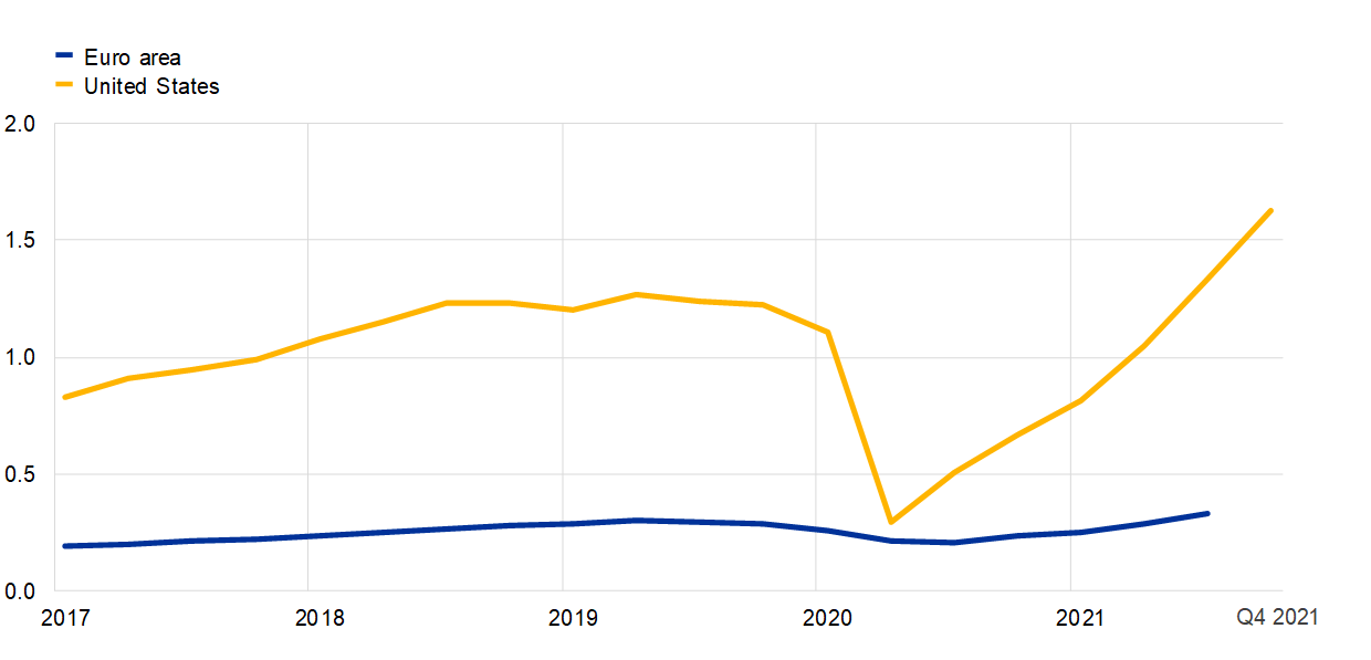
Chart 1 shows the evolution of core inflation in both the euro area and the United States. The evolution of headline inflation is dominated by the extraordinary rise in energy prices, with further upward pressure recently from food prices. At a qualitative level, there has been a significant pickup in core inflation in both monetary areas, even if the quantitative scale of the increase is quite different. The impact of the pandemic on core inflation can be split into two categories: (i) those goods and services affected by supply disruptions and bottlenecks; and (ii) those goods and services affected by re-opening disruptions (primarily high-contact services). The bottlenecks category has put upward pressure on core inflation in both the euro area and the United States but the quantitative impact has been substantially larger for the United States.
Chart 1
Inflation excluding food and energy in the euro area (left panel) and United States (right panel)
(annual percentage changes and percentage point contributions)
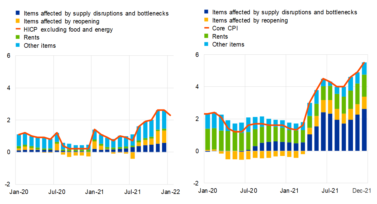
Sources: Eurostat, Haver and ECB staff calculations.
Notes: For the euro area, the panel shows the HICP excluding food and energy, as well as the contributions to it. For the United States the panel shows the CPI excluding food and energy, as well as the contributions to it. Items affected by bottlenecks include new motor cars, second-hand motor cars, spare parts and accessories for personal transport equipment, and furnishings and household equipment. Items affected by reopening include clothing and footwear, recreation and culture, recreation services, hotels and motels, and domestic and international flight prices. Rents include actual rents paid by tenants, and for the United States also imputed rents for owner-occupied housing. The latest observations are for January 2022 for HICP excluding food and energy in the euro area, otherwise December 2021.
A basic reason why the scale of inflation linked to bottlenecks has differed between the euro area and the United States is that the overall impact depends on the scale of the mismatch between supply and demand. Chart 2 shows the dynamics of consumption for the euro area and the United States. While consumption is only now approaching pre-pandemic levels in the euro area, overall consumption in the United States had recovered by spring 2021. There was also a remarkable relative shift from services towards goods, especially durable goods. While there was also a relative expenditure shift toward goods in the euro area, the scale of demand for goods was of a different order of magnitude in the United States.
Chart 2
Real consumption expenditure in the euro area (left panel) and United States (right panel)
(left panel: index: Q4 2019 = 100; right panel: index: December 2019 = 100)

Sources: Eurostat and ECB staff calculations for the euro area, and US Bureau of Labor Statistics and ECB staff calculations for the United States.
Note: The latest observations are for the third quarter of 2021 for the euro area and December 2021 for the United States.
Chart 3 focuses on the impact of supply bottlenecks on non-energy industrial goods (NEIG) inflation in the euro area, using two different empirical techniques. Both approaches show that the bottleneck component of NEIG inflation has been visible since about February 2021 and has been broadly stable since summer 2021. In terms of scale, the two approaches differ but suggest that supply bottlenecks contributed about 20-50 basis points to NEIG inflation in the euro area.
Chart 3
Impact of supply bottlenecks on inflation in non-energy industrial goods (NEIG) in the euro area
(percentage points)
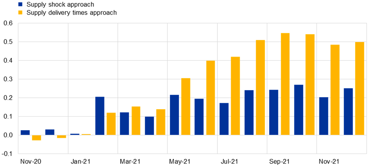
Sources: Eurostat, Markit and ECB staff calculations.
Notes: Effects of supply bottlenecks on HICP NEIG are estimated using two VARs that include HICP NEIG inflation, producer prices, industrial production, export and import values plus (1) a supply shock (“two-step supply shock approach”) or (2) supply delivery times (“one-step supply delivery times approach”) as a proxy for supply-side constraints. The supply shock is estimated from a first-stage bivariate VAR using PMI output and supply delivery times and applying sign restrictions. For each approach, the marginal effect of supply bottlenecks is derived by taking the difference between a conditional and counterfactual VAR forecast. The latest observations are for December 2021.
In Chart 4, some indicators of global bottleneck pressures are shown. The chart shows that supplier delivery times (according to Purchasing Managers’ Index (PMI) surveys) have been broadly stable at the global level over the past year – while this indicator of supply disruptions has not deteriorated over this period, it has not markedly improved either.[6] At a geographical level, some rotation is visible: supplier delivery times have shortened for the most-affected countries (the United Kingdom and the United States) but have lengthened (albeit from a much lower base) for Japan.
Chart 4
Global economic activity: supplier delivery times
(diffusion index)
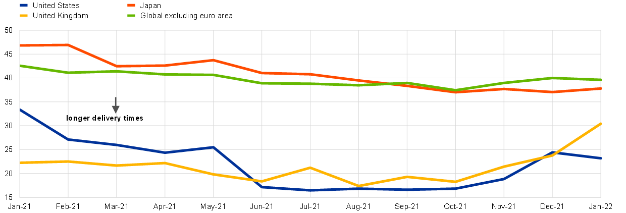
Sources: Markit and ECB staff calculations.
Note: The latest observations are for January 2022.
Chart 5
Global economic activity: shipping rates (left panel) and volumes (right panel)
(left panel: spot rates in USD; right panel: weekly cargo volumes in 20-foot equivalent units)
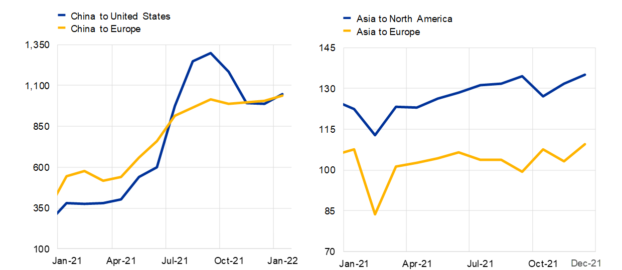
Sources: WSTS and Bloomberg.
Note: The latest observations are for January 2022 for prices and December 2021 for volumes.
Chart 5 shows that there was a sizeable increase in shipping prices in the first half of 2021, which was particularly sharp for shipping from China to the United States. Shipping prices from China to Europe stabilised in the second half of 2021, but have not declined, whereas shipping prices from China to the United States have fallen back to a level that is now similar to the China-Europe route. The right panel of Chart 5 shows that shipping volumes increased significantly during 2021, despite serious interruptions to supply capacity due to the Suez Canal incident and geographical mismatches in container availability: the bottleneck phenomenon in relation to shipping was exacerbated by the rapid increase in demand for manufactured goods and commodities, especially from the United States.
Taking a broader view of supply-side constraints in the euro area, Chart 6 graphs a synthetic aggregate indicator of bottlenecks (based on a dynamic factor model that combines a range of measures), together with the PMI index of manufacturing supplier delivery times.[7] In turn, Chart 7 shows a heat map of the various individual measures used in the dynamic factor model. The overall message from Charts 6 and 7 is that there was a significant increase in supply disruptions over the course of 2021 but the impetus in terms of the levels effect had largely stabilised by the end of the year. However, the PMI indicator (which is constructed to be forward looking) has noticeably declined since late 2021, which suggests that some easing of supply disruptions can be expected.
Chart 6
Supply chain pressures
(left-hand scale: standard deviations from long-term mean; right-hand scale: diffusion index)

Sources: Markit and ECB staff calculations.
Notes: Higher values denote longer delivery times. The dynamic factor model is computed including all indicators listed in Chart 7 and excluding the PMI suppliers’ delivery times. The latest observations are for January 2022.
Chart 7
Heat map of sectoral indicators used to monitor supply bottlenecks
(z-scores)
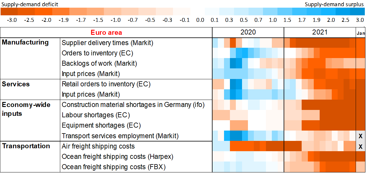
Sources: European Commission (EC), Markit, Harpex, Freightos Baltic Index (FBX), ifo Institute, and ECB staff calculations,
Notes: The heatmap shows z-scores, which are computed by subtracting the mean from the observation at time t and dividing the obtained difference by the standard deviation. Mean and standard deviation are computed over the available sample from January 1999 to January 2022. Positive (negative) values represent how many standard deviations the index is above (below) the average value. Transportation costs and commodities prices are in year-on-year growth rates. Some z-scores are multiplied by -1 (i.e. prices) consistently with the concept of supply and demand pressures. The source is provided in the heatmap for soft indicators. Observations marked with an X are not available. The latest observations are for January 2022.
In terms of other signals about the future course of supply disruptions, Chart 8 plots the answers from the ECB’s latest corporate telephone survey. While the survey does indicate that bottleneck pressures are expected to ease, this will take some time – the modal answer in the survey was that bottlenecks would persist for at least another six months. While around a quarter of respondents were more optimistic (predicting that bottlenecks would ease within six months), another quarter of respondents feared that bottlenecks would persist for about a year.
Chart 8
Expected persistence of supply bottlenecks: results from the corporate telephone survey
(percentage of respondents)
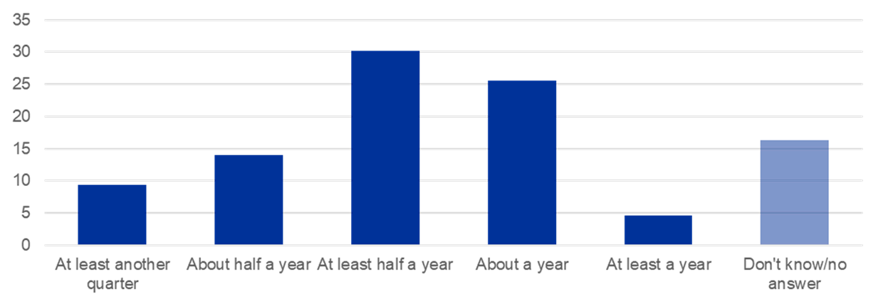
Source: Corporate telephone survey, January 2022.
As regards the energy sector, supply-side disruptions are playing a role in the surge in energy prices.[8] While it is beyond the scope of this blog post to provide a full analysis of the drivers of energy price dynamics, Chart 9 presents a decomposition of oil prices since the start of the pandemic. Although the pandemic-related decline in global economic activity goes a long way in explaining the plunge in oil prices in 2020, the subsequent surge in the oil price beyond its pre-pandemic level is mainly attributable to supply-side factors. Supply constraints may in part relate to the carbon transition, but production disruptions in some regions, OPEC+ supply strategies and the spillover impact on oil coming from supply disruptions in the gas market are also playing a role.
Chart 9
Oil price decomposition
(cumulative percentage changes since January 2020)

Sources: Refinitiv and ECB staff calculations.
Notes: Structural shocks are estimated using the spot price, the futures to spot spread, market expectations of oil price volatility and the stock price index. Based on Venditti, F. and Veronese, G., (2020). Global Financial Markets and Oil Price Shocks in Real Time. ECB Working Paper No. 20202472. The latest observations are for 31 January 2022.
For gas prices, the left panel of Chart 10 shows that their volatility is inversely related to the level of inventories. In particular, a shock that might have little impact on gas prices when inventories are high can exert a significant impact when inventories are low. This basic non-linearity helps to explain the very high volatility seen in the gas market in recent months. The right panel reflects this volatility along two dimensions. First, compared to the gas price profile that was incorporated in the staff macroeconomic projections in December 2021, the spot price of gas has declined considerably in recent weeks. Second, at the same time, there has been a significant revision in the futures curve, especially for the current year. Although a significant decline in gas prices is still expected, the timing has been shifted outwards, with the scale of declines during 2022 priced to be much more muted compared to the December 2021 projections exercise. Of course, it should be emphasised that futures prices also incorporate risk premia, so these do not necessarily capture a “true” expectation of future prices, and geopolitical tensions (together with weather-related uncertainty) mean that risk considerations are especially pertinent at the moment.
Chart 10
Gas prices: price effects of gas supply shocks (left panel) and outlook for European gas prices (right panel)
(left panel: price effect after six months, percentages; right panel: EUR/MMBtu)
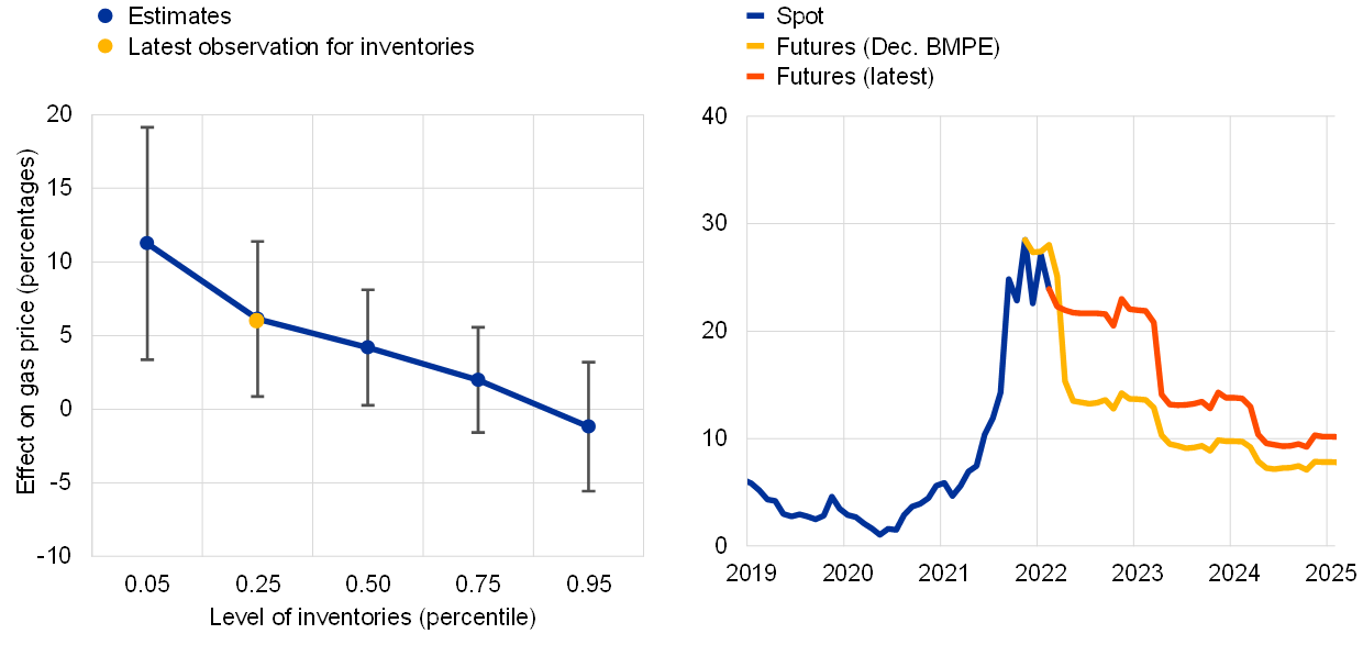
Sources: Refinitiv, IEA and ECB staff calculations for the price effects of gas price shocks, and Refinitiv and Bloomberg for the outlook for European gas prices.
Notes: Gas price supply shocks are estimated from a three variable BVAR including the European gas price (Dutch TTF price), gas consumption and industrial production. Shocks are identified using sign restrictions, with a supply shock assuming that gas prices rise while gas consumption and industrial production fall. For the price effects of gas price shocks, the vertical axis shows percentage increases in gas prices following shocks at a six-month horizon. The horizontal axis shows the level of inventories, which is measured as the residual of a regression of log inventories on calendar months to remove seasonal effects. Other control variables include the lag dependent variable, three lags of the VIX, and supply, demand and economic activity shocks and an interaction of the shock on interest and the level of inventories. The sample period is November 2008 to September 2021. The current level of inventories is in the 20th percentile of the distribution (see yellow dot). For the outlook for European gas prices, Spot refers to Dutch TTF, MMBtu = million British thermal units, and BMPE stands for Eurosystem staff Broad Macroeconomic Projection Exercise. The latest observations are for 31 January 2022.
Turning to the labour market, Chart 11 shows the recent dynamics of certain earnings indicators in the euro area and the United States. Although earnings growth in the euro area remains muted so far (as tracked by negotiated wages), there has been a significant increase in average hourly earnings in the United States. Chart 12 shows that the euro area labour market has made considerable progress in recent months, with the labour force participation rate back to pre-pandemic levels, unemployment declining to 7.0 percent (faster than expected in the December 2021 staff projections) and the PMI employment indicators signalling employment growth across all sectors.
Chart 11
Wage developments: euro area negotiated wages (left panel) and US average hourly earnings (right panel)
(annual percentage changes)

Sources: Eurostat and ECB staff calculations for euro area negotiated wages, and the US Bureau of Labor Statistics, US Bureau of Economic Analysis and ECB calculations for US average hourly earnings.
Notes: For euro area negotiated wages, the fourth quarter of 2021 is based on October and November data for the euro area. For US average hourly earnings, the grey boxes show the interquartile range, i.e. the range between the 25th and 75th percentile over the period from the first quarter of 1997 to the fourth quarter of 2019. The whiskers indicate the minimum and maximum data, excluding outliers.
At the same time, the euro area labour market is not experiencing the same degree of labour market tightness as in the United States. Chart 12 shows the ratio of vacancies to unemployment. While this is ticking up in the euro area and is higher than before the pandemic, the level of this ratio is far higher and its slope has been far steeper in the United States. Other indicators also suggest that the labour market has not fully recovered. Hours worked in the euro area are still below the pre-pandemic level and various furlough and wage subsidy schemes remain in place, so the overall state of the labour market continues to be affected by pandemic-related factors. In addition, there is still the important open question of whether the degree of entry by foreign workers (which is especially important in the services sector) will return to pre-pandemic levels once the pandemic is behind us.
Chart 12
Labour market tightness in the euro area and United States
(job vacancy rate divided by the unemployment rate)
Source: ECB staff calculations based on data from Eurostat and the US Bureau of Labor Statistics.
Notes: The latest observations are for the fourth quarter of 2021 for the United States and the third quarter of 2021 for the euro area.
Still, the improvement in the labour market indicates that wage dynamics should strengthen over the course of 2022-2024. A marked pickup was already incorporated in the December staff projections, while the latest corporate telephone survey also suggests that wages are expected to grow more quickly during 2022, as is shown in Chart 13. Although this survey focuses on large firms, and therefore does not represent the full spectrum of the labour market, it does provide a directional guide to wage pressures across a significant number of sectors and countries.
Chart 13
Contacts’ assessment of average wage growth: results from the corporate telephone survey
(annual percentage change)
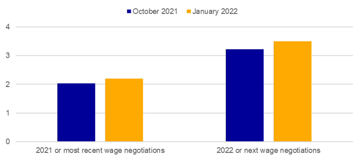
Source: Corporate telephone survey.
Conclusion
In this blog post, I have covered three categories of bottlenecks: (i) tradable goods; (ii) energy; and (iii) the labour market. Since the prices of tradable goods and energy are heavily influenced by global factors, supply-demand mismatches that originate in external factors can exert a powerful impact on the overall inflation rate. However, bottleneck-related price pressures should fade over time as pandemic-induced frictions disappear and supply and demand adjust in response to relative price movements.
In relation to the labour market, a bottleneck scenario can emerge if there is an unexpected and large-scale increase in aggregate labour demand or a substantial shortfall in aggregate labour supply. Although there might be some signs of labour market bottlenecks in certain sectors in some euro area countries, the overall profile of the euro area suggests a smooth recovery in overall labour supply (even if the scale of the future return of foreign workers remains an open question) and provides hopeful signs of a gradual-but-sustained increase in labour demand. Such a gradual tightening of the labour market constitutes a key mechanism for inflation to stabilise at our two per cent target over the medium term, whereas there are no indications of aggregate overheating in the euro area labour market.
- This blog post serves as background material for my contribution to the roundtable on supply chains at EU Industry Days 2022 on 10 February 2022.
- In turn, supportive monetary policies, macroprudential policies and supervisory policies provided strong underpinnings for monetary and financial stability, avoiding that the adverse pandemic shock would be amplified by disinflationary pressures or excessive tightening of financing conditions.
- Bottleneck pressures have also been generated by an assortment of other shocks, including weather shocks. The insufficient resilience of global supply chains and logistics networks has also been a contributory factor.
- See, for example, Guerrieri, V., Lorenzoni, G., Straub, L. and Werning, I. (2021), “Monetary Policy in Times of Sectoral Reallocation”, contribution to the 2021 Jackson Hole Economic Policy Symposium. In addition to cyclical relative price shocks, a similar logic suggests an increase in relative price trends should be reflected in a higher inflation target (Adam, K. and Weber, H. (2021), “Estimating the Optimal Inflation Target from Trends in Relative Prices”, American Economic Journal: Macroeconomics, forthcoming).
- European producers of manufactured goods that are sold on international markets or rely on imported inputs may also respond to global bottlenecks by raising prices. This way the external shock may generate increases in domestic producer prices and export prices. Accordingly, external bottlenecks may be one factor behind the observed increase in producer prices in the euro area. In turn, the resolution of external bottlenecks may also affect the subsequent evolution of domestic producer prices and export prices.
- The chart focuses on 2021. Supplier delivery times had already been disrupted by the pandemic during 2020.
- The Global Supply Chain Pressure Index developed by a team of economists at the Federal Reserve Bank of New York tells a similar story. See G. Benigno, J. di Giovanni, J. J. J. Groen, and A. I. Noble (2022), “A New Barometer of Global Supply Chain Pressures,” The Liberty Street Blog (4 January 2022).
- The very large swing in oil prices has been a primary contributor to the very low inflation outcome in 2020 (0.3 percent) and the increase in inflation from this low base in 2021. Since much of the oil price increase occurred in the final months of 2021, base effects (comparing current oil prices versus oil prices twelve months ago) will still push up measured annual inflation for much of 2022.