- RESEARCH BULLETIN NO. 59
- 27 June 2019
Price and Wage Setting when Accurate Decisions Are Costly: Implications for Monetary Policy Transmission
Recent low inflation is motivating new research to better characterise how individual firms and workers set prices and wages. In this article, we describe a new approach which emphasises that the costs of decision-making may limit the precision of price and wage changes. As well as making better sense of price and wage changes in microeconomic data, this new approach also strikes a middle ground between two leading models of monetary policy transmission, improving our quantitative understanding of the short-run effects of monetary policy on output and the short-run trade-off between inflation and unemployment.
Understanding inflation and the effects of monetary policy requires an understanding of the way in which firms and workers set prices and wages. Motivated by the current low inflation environment, this article discusses ongoing research on modelling price and wage setting at the level of individual firms and workers. It then traces out the macroeconomic and policy implications of this new modelling approach for understanding how monetary policy is transmitted to inflation and output.
Most models used to analyse monetary policy issues today rely on the assumption that nominal prices are “sticky”, meaning that they adjust relatively infrequently. For example, a brand of bread that costs €1.79 per loaf today is very likely to still cost exactly €1.79 next week. However, existing models of price stickiness have a number of shortcomings. The most widely-used approach, the model of Calvo (1983), assumes that prices change intermittently, at entirely random times. Given that randomness, the Calvo model offers no insight into the trade-offs firms face in deciding when to change their prices. Other models have relied on “menu costs”: these models assume that a firm must pay a fixed cost whenever it wishes to adjust a price (see Golosov and Lucas, 2007). However, the menu cost approach is hard to reconcile with price changes observed in microeconomic data on retail firms. Moreover, menu cost models generate a very flexible aggregate price level, implying speedy transmission of monetary policy to inflation and hence much smaller “real” effects of monetary policy than the Calvo model predicts.[2] These implications of the menu cost approach conflict with some empirical evidence showing a rather gradual inflation response to changes in the central bank’s monetary policy stance, and a relatively large and persistent response of real output.
Finding the right model of price adjustment is not an idle academic question, since different approaches have very different implications for the impact of monetary policy. Therefore, ongoing research is seeking alternatives to the Calvo and menu cost approaches that can better match features of retail price microdata and better explain how decisions to adjust prices and wages vary with prevailing economic conditions. We have developed a new approach that highlights the exorbitant cost of making choices with perfect accuracy. This framework, known as “control costs”, posits that making more accurate decisions is more costly, so achieving perfect precision by selecting the “best” price at exactly the “best” time is unlikely to be optimal.[3] This idea is in line with evidence from case studies, e.g. Zbaracki and co-authors (2004), which suggests that the time managers and employees spend making decisions is a large component of the costs of price-setting. In addition, recent experimental evidence points to errors in the timing of adjustment by decision-makers (Khaw, Stevens and Woodford, 2016).
The control cost model covers the range of possible degrees of “state-dependence” in monetary policy transmission, from the fixed menu cost model (at one extreme) to the Calvo model (at the other extreme). The fixed menu cost (FMC) extreme represents infinite precision (zero control costs), so that price adjustments are fully optimal, responding fully to the state of the firm and the economy. The Calvo model amounts to zero precision (infinite control costs) in timing, so that the timing of price adjustments is totally random, regardless of the situation. As a consequence, the real effects of monetary shocks are smallest in the FMC model and largest in the Calvo model. In all these respects, the control cost model occupies a middle ground between the other two models, and we find when we estimate its parameters that it appears compatible with microeconomic and macroeconomic evidence simultaneously.
Figure 1
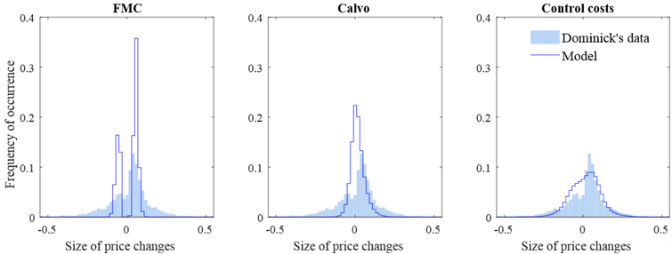
Distribution of price changes: Price-setting models versus the data

Notes: Solid blue lines show the probability of price changes of different sizes predicted by each of the models. Blue shaded areas show the actual price changes observed in the Dominick’s Finer Foods database, as documented by Midrigan (2011).[4] Source: Costain and Nakov (2019), Fig. 3.
On the microeconomic side, consider Figure 1, which compares the predicted frequency of price changes of various sizes in the control cost model, the Calvo model, and the FMC model to the pattern of price changes observed in data from a chain of retail stores. The blue lines show the predicted price changes; the blue shaded area shows the actual price changes. The FMC and Calvo models are at odds with the actual data, where some very tiny price changes coexist with some very large ones. The FMC model predicts very few small price changes, because it implies that a price is adjusted exactly at the moment when its deviation from the optimal value becomes large enough to justify paying the fixed cost. At the opposite extreme, since adjustment timing in the Calvo model is completely random, many price changes turn out to be extremely small. In contrast, our control cost framework better matches the entire range of small and large price changes observed in the data. This improvement in model performance occurs because with control costs, perfect accuracy in price-setting is excessively costly, so firms tolerate some errors both in the timing of price adjustments, and in the new levels at which prices are set. This spreads out the range of predicted price changes, resembling the widely dispersed distribution observed in the data.
Figure 2
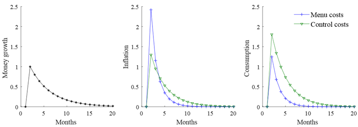
Effects of money growth shocks across pricing models

Notes: Responses of inflation and consumption to a persistent money growth shock. Blue line: Fixed menu cost model. Green line: Control cost model, applied to prices only. Vertical axis shows percentage point deviation (money growth; inflation) and per cent deviation (consumption) from steady-state values. Source: Costain and Nakov (2019), Fig. 6.
Taking account of human cognitive limits not only helps interpret adjustment patterns in microeconomic data on individual firms; it also helps explain macroeconomic evidence that inflation responds relatively slowly to changes in the monetary policy stance while real output responds significantly in the short run. Figure 2 compares the effects of a sudden and unexpected increase in money growth on inflation and private consumption in the control cost model (green line) and in the FMC model (blue line). It shows that the FMC model generates an immediate burst of inflation in response to this policy change, and a relatively muted and brief response of consumption. In contrast, under control costs, the effect on inflation is initially only half as large, but it is more persistent, giving rise to a long-lasting decline in the real interest rate that generates a stronger and more persistent impact on consumption. The differences reflect errors in the timing of price changes, which slow down the inflation response and increase the real effects on consumption. In other words, control costs inject randomness into the adjustment timing, muting the strong “selection effect” found with the FMC model. Thus, our new model helps to reconcile micro price-setting patterns with empirical macro evidence that monetary stimulus has a substantial short-run effect on output, followed by a somewhat delayed and persistent response of inflation.
Figure 3
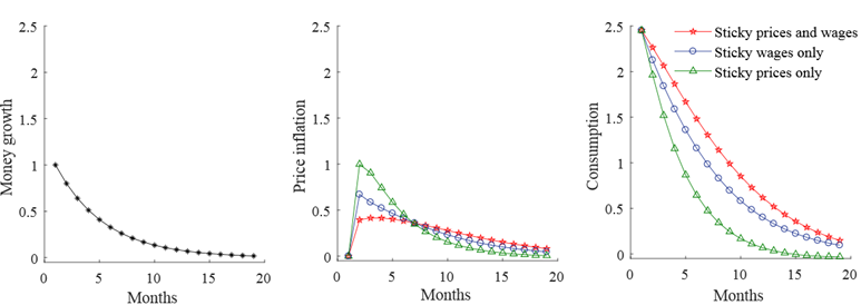
Effects of money growth shocks with price and/or wage stickiness

Notes: Responses of inflation and consumption to a persistent money growth shock in several versions of the control cost model. Green: Control costs affecting prices only. Blue: Control costs affecting wages only. Red: Control costs affecting prices and wages. Vertical axis shows percentage point deviation (money growth; inflation) and per cent deviation (consumption) from steady-state values. Source: Costain, Nakov, and Petit (2019), Fig. 8.
The control cost framework can also be applied to modelling wage setting. Figure 3 compares the effects of an unexpected increase in money growth in model variants with sticky prices only, with sticky wages only, and then with both sticky prices and sticky wages. It shows that sticky wages generate a more gradual and persistent inflation response than sticky prices do. Relatedly, if wages are sticky, then the short-run real effects of a money growth shock on consumption are larger and longer-lasting. This is partly because wages are adjusted less frequently than prices, on average (both in the model and in the data), and also because wages are a major component of costs, and are therefore a major driver of prices. These findings suggest that the real effects of monetary policy may depend more on wage rigidities than on price rigidities per se, and imply that monitoring wage developments is crucial for appropriate monetary policy decisions.
Figure 4
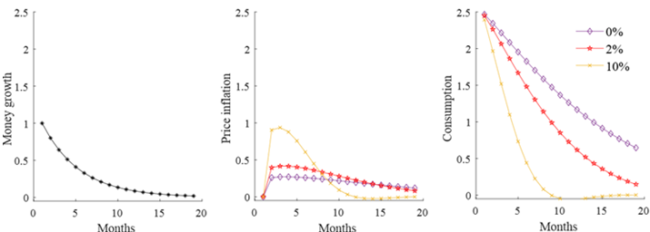
Effects of money growth shocks at different trend inflation rates

Notes: Responses of inflation and consumption to a persistent money growth shock in the control cost model, starting from different trend inflation rates. Purple: 0% trend inflation. Red: 2% annual trend inflation. Yellow: 10% annual trend inflation. Vertical axis shows percentage point deviation (money growth; inflation) and per cent deviation (consumption) from steady-state values. Source: Costain, Nakov, and Petit (2019), Fig. 11.
Finally, unlike the Calvo framework, our model implies that both the frequency and the size of changes in prices and wages will depend on the longer-run “trend” rate of inflation. In the current environment of prolonged low inflation, both price and wage adjustments should become smaller and less frequent. In turn, this implies that changes in the monetary policy stance will have a smaller impact on inflation, and will instead have larger real effects on consumption, employment, and output. The largest real effects occur when trend inflation is zero; they are slightly smaller at either plus or minus one per cent trend inflation. Figure 4 shows that the real effects of monetary policy shocks become much less persistent as trend inflation rises from 0% to 2% and to 10% per annum.[5] Hence, in our model, the episode of persistently low inflation in recent years helps explain the flatter Phillips curve observed over the same period.[6] Our results also emphasise the continued relevance of monetary policy for stabilising the real macroeconomy.
References
Calvo, G. (1983), “Staggered prices in a utility-maximizing framework,” Journal of Monetary Economics Vol. 12, September, pp. 383-398.
Costain, J. and Nakov, A. (2019), “Logit price dynamics,” Journal of Money, Credit and Banking Vol. 51, No. 1, February, pp. 43-78.
Costain, J., Nakov, A. and Petit, B. (2019), “Monetary Policy Implications of State Dependent Prices and Wages”, ECB Working Paper No. 2272, April.
Golosov, M. and Lucas, R. (2007), “Menu costs and Phillips curves,” Journal of Political Economy Vol. 115, No. 2, April, pp. 171-199.
Khaw, M. W., Stevens, L., and Woodford, M. (2017), “Discrete adjustment to a changing environment: Experimental evidence.” Journal of Monetary Economics Vol. 91, November, pp. 88-103.
Mattsson, L.-G. and Weibull, J. (2002), “Probabilistic choice and procedurally bounded rationality,” Games and Economic Behavior Vol. 41, No. 1, October, pp. 68-71.
Midrigan, V. (2011), “Menu costs, multiproduct firms, and aggregate fluctuations,” Econometrica Vol. 79, No. 4, July, pp.1139-1180.
Zbaracki, M. J., Ritson, M., Levy, D., Dutta, S. and Bergen, M. (2004), “Managerial and customer costs of price adjustment,” Review of Economics and Statistics Vol. 86, No. 2, May, pp. 514-533.
- Disclaimer: The article was written by James Costain (Economist, DG Research) and Anton Nakov (Economist, DG Research). The authors thank Michael Ehrmann, Geoff Kenny, Philipp Hartmann, and Alberto Martín for helpful advice. The views expressed here are those of the authors and do not necessarily represent the views of the European Central Bank and the Eurosystem.
- The reason for this is a strong “selection effect”, whereby those prices that are most misaligned are the ones which are re-optimised. This implies relatively large absolute price changes on impact when a monetary policy change occurs, leading to a highly flexible aggregate price level and hence small real effects of the policy change.
- The “control cost” framework was originally developed in game theory, where it helped explain apparent errors made by participants in economic laboratory experiments (see Mattsson and Weibull, 2002). We have adapted this framework to describe decisions by firms and workers in a macroeconomic model.
- Data source: James M. Kilts Center, University of Chicago Booth School of Business. The Dominick’s Finer Foods database covers a limited sub-set of all the goods represented in the CPI. However, size histograms of price changes from other sources, e.g. AC Nielsen, display a similar roughly bell-shaped, slightly bimodal, pattern.
- The “half-life” of the consumption response falls from 10 months at 0% trend inflation to seven months in the baseline simulation, which features 2% trend inflation; and it falls to four months at a 10% trend inflation rate.
- The Phillips curve is a short-term relationship between the rate of inflation and the rate of (un)employment.


