
Measures of underlying inflation for the euro area
Measures of underlying inflation for the euro area
Published as part of the ECB Economic Bulletin, Issue 4/2018.
Headline inflation can be noisy, blurring the signal on the medium-term inflationary pressure relevant for monetary policy. To help distinguish signal from noise in the data, central banks monitor measures of underlying inflation. As there are many ways of measuring underlying inflation, it is important to understand the properties of the various indicators and what factors may account for any divergence between them. This article describes in detail the measures of underlying inflation typically used at the ECB and evaluates them against a set of empirical criteria.
1 Introduction
Central banks should be mainly concerned with persistent sources of inflationary pressure and less so with short-lived, reversible movements in the inflation rate. The price stability objective of the Eurosystem is to maintain annual rates of headline HICP (Harmonised Index of Consumer Prices) inflation at below, but close to, 2% over the medium term. As HICP inflation comprises a broad-based basket of goods and services, developments in the annual rate of HICP inflation may be temporarily influenced by factors that are mainly of a short-term nature. These factors can include price changes that stem from volatility in, for example, commodity prices, or price changes that are not determined by market forces, such as those in administered prices, as well as price changes that are specific to certain product markets. Such short-term changes may be looked through, in particular if they are not likely to lead to second-round effects.
The central bank faces the problem of distinguishing in real time the “signal” on medium-term inflationary pressure contained in the HICP inflation data from the “noise” stemming from temporary or idiosyncratic factors. To this end, measures of underlying inflation are routinely monitored. Generally, their purpose is to obtain an estimate of where headline inflation will settle in the medium term after temporary factors have vanished. This is conceptually akin to estimating the evolution of the (unobservable) persistent component of headline inflation, which will be simply referred to in what follows as “trend inflation”.[1] Operationally, this estimation can be performed at various levels of statistical complexity, ranging from excluding some components of headline inflation a priori on account of their volatility, through taking simple moving averages of headline inflation, to estimating complex statistical models that exploit the cross-sectional variation of inflation components. Underlying inflation measures can provide intermediate verifiable milestones, together with a broader set of macroeconomic information, to assess medium-term inflationary pressure. In practice, as any measure of underlying inflation is inherently surrounded by a large degree of uncertainty, for the purposes of robustness central banks use a wide range of measures (see Box 1).
The assessment of developments in measures of underlying inflation requires an appreciation of their respective properties and needs to be followed up by an examination of the economic forces driving inflation. Alternative measures of underlying inflation may provide conflicting signals, as has been the case over recent years. This brings back into focus the need to review their relative properties, on the basis of both conceptual and empirical criteria. It is also worth stressing that the measures of underlying inflation provide only a first-pass, often only statistical-based, perspective on medium-term inflationary pressure. A conjunctural assessment of developments in measures of underlying inflation needs to be followed up by an examination of the driving forces in order to better understand the inflation process, but this is beyond the scope of this article.[2]
Against this background, this article discusses the measures of underlying inflation used at the ECB and evaluates their properties against a set of empirical criteria. To extract an overall assessment that can support policymakers, it is not enough to just compare developments in alternative indicators: one must also clearly understand their properties under different macroeconomic circumstances and benchmark them against a well-defined set of metrics. To this end, Section 2 describes the conceptual properties of the measures of underlying inflation typically used at the ECB and Section 3 evaluates these measures against a set of empirical criteria. Section 4 concludes.
Box 1 The use of measures of underlying inflation at selected central banks
Central banks typically formulate their price stability objectives in terms of headline inflation. This mostly follows welfare considerations. It is the preservation of the purchasing power of the currency, as measured by the most representative and comprehensive price index, that matters for consumers. While they may capture the broad inflation trends, measures of underlying inflation do not represent the cost of living and, as such, they may not be readily accepted by the public as an objective of monetary policy. For the selected central banks shown in Table A, the inflation aim is generally defined in terms of headline CPI (Consumer Price Index) inflation. However, the US Federal Reserve focuses on Personal Consumption Expenditure (PCE) inflation, which is an index covering a wide range of household spending, while Sveriges Riksbank recently adopted a CPI measure that excludes the effects of changes in household mortgage rates (the CPIF).[3] Table A shows that most advanced economies’ central banks have a 2% aim for headline inflation, with the Reserve Bank of Australia and the Reserve Bank of New Zealand having target ranges.
Table A
Price stability objectives and measures of underlying inflation of selected central banks

Sources: Central bank websites; FOMC statement of longer-run goals and policy strategy, press release, Federal Reserve, 25 January 2012; The “Price Stability Target” under the Framework for the Conduct of Monetary Policy, Bank of Japan, 22 January 2013; Monetary policy remit: Autumn Budget 2017, HM Treasury, 22 November 2017; Renewal of the Inflation-Control Target – Background Information, Bank of Canada, October 2016; 2016 Statement on the Conduct of Monetary Policy, Reserve Bank of Australia and Australian Government, 19 September 2016; and Policy Targets Agreement 2018, Reserve Bank of New Zealand and Ministry of Finance, 26 March 2018. The classification in the last column partly follows Table 1 in Kahn, M., Morel, L. and Sabourin, P., “A comprehensive assessment of measures of core inflation for Canada”, Bank of Canada Discussion Paper 2015‑12, 2015.
Measures of underlying inflation, which abstract from short-term volatility, are typically monitored by central banks to gauge trends in inflation and the likely evolution of inflation in the medium term. While the emphasis on individual measures of underlying inflation tends to change over time, the most commonly used measures are those that exclude the components with more volatile price movements (see Table A), possibly because they are easier to replicate and communicate to the public. Measures based on trimmed means and weighted medians are also fairly commonly used, whereas model-based measures, such as those derived from factor models and principal component analysis, tend to be referred to less often in central banks’ official communication.
The specific measures of underlying inflation that are used tend to vary across different central banks. The Federal Reserve, for example, regularly monitors core inflation, in particular the PCE price index excluding food and energy, as a measure providing a better indication than the headline figure of where overall inflation will be in the future.[4] The Bank of Japan looks at four measures of underlying inflation, obtained by removing transitory disturbances from the actual movements observed in consumer prices, as a way to identify trends in price movements.[5] The Bank of England has recently discussed various exclusion-based measures of inflation as approximations for domestically generated inflationary pressure.[6] The Bank of Canada explicitly uses three measures of core inflation as “operational guides” to achieve the total CPI inflation target, but not as a replacement for it.[7] Norges Bank monitors a range of (mostly exclusion-based) measures as a way to look through temporary variations in inflation. For these measures, it also produces forecasts over the policy-relevant horizon. All central banks interpret the various measures of underlying inflation in conjunction with other available information about broader economic developments.
Measures of underlying inflation are referred to in the official communication of central banks. Based on a textual analysis of the official policy statements issued by the Federal Open Market Committee (FOMC) of the Federal Reserve and the Governing Council of the ECB between October 1998 and March 2018, Chart A displays the number of times that expressions related to underlying inflation appear in the official policy statements of the two institutions. Both seem to make low to moderate use of the concept in their official communication, with the ECB referring to it, on aggregate, slightly more often than the Federal Reserve, even when accounting for the higher number of policy statements issued during the period (218 introductory statements for the ECB and 165 statements for the FOMC). Looking at the occurrence of different expressions conveying the notion of underlying inflation, Chart A shows that the ECB typically refers to “underlying inflation” and “underlying price pressure”, while terms like “inflation trend” and “core inflation” recur more frequently in the communication of the Federal Reserve.
Chart A
References to underlying inflation terms in the official communication of the ECB and the Federal Reserve
(number of occurrences)

Source: ECB calculations.
Notes: The period covered is October 1998 to March 2018. The two bars on the left-hand side refer to the total number of references and equal the sum of all categories on the right-hand side. The sample includes 218 ECB introductory statements and 165 FOMC statements.
As a further step, it is interesting to see whether the use of the concept of underlying inflation in central bank communication displays any regularity, for example appearing more frequently in periods during which price developments are not aligned with the inflation aims of the central banks. Chart B provides tentative evidence that the ECB and the Federal Reserve have referred to underlying inflation both in times of high and low headline inflation, with the ECB using the concept slightly more often when inflation is low and the Federal Reserve when inflation is high. Neither central bank seems to make more intensive use of the concept during episodes of significant deviations of headline inflation from their respective inflation aims.
Chart B
Headline inflation and references to underlying inflation in the official communication of the ECB and the Federal Reserve
(annual percentage changes)

Sources: Federal Reserve Bank of St. Louis, Eurostat and ECB calculations.
Notes: The y-axis shows the annual percentage change in headline HICP inflation for the ECB and in US PCE inflation for the Federal Reserve. The period covered is October 1998 to March 2018.
2 Measures of underlying inflation
There are many ways to measure underlying inflation.[8] Although quite diverse methods are used in their construction, measures of underlying inflation generally have the common aim to filter out the short-term volatility in headline inflation in order to capture the low-frequency component of inflation in a timely manner. The measures of underlying inflation typically used at the ECB can be sub-divided into three broad categories: permanent exclusion measures, temporary exclusion measures, and frequency exclusion measures. This section describes the conceptual nature of and the methodologies behind these measures, taking each category in turn. In particular, the rationale behind the measures is highlighted, while the desirable empirical properties, such as smoothness and the ability to track trend inflation, are evaluated in the next section.
The first class of measures permanently removes certain volatile sub-components. Volatility in headline inflation can sometimes be attributable to temporary factors that have little relevance for the medium-term outlook. For example, oil prices often exhibit large swings that can produce, over the short term, substantial direct effects on energy prices. Similarly, unseasonal weather can sometimes induce strong volatility in unprocessed food prices. To abstract from such volatility, HICP inflation excluding energy and food (HICPX) is often used as a measure of underlying inflation. However, the HICPX inflation rate can still reflect the influence of substantial transitory effects, as was evidenced during the spring of 2017 when Easter-related calendar effects were behind large fluctuations in the annual HICPX inflation rate (see Chart 1). In addition, the price signal for clothing and footwear may be unduly influenced by the timing of the sales periods. To abstract from these factors, the inflation rate for HICPX excluding travel-related items, clothing and footwear is also tracked at the ECB.[9],[10] During 2017 there was a notable but temporary divergence between this measure and HICPX, which was mainly attributable to the impact of higher inflation for the volatile travel-related items sub-component.[11]
Chart 1
Exclusion-based measures of underlying inflation
(annual percentage changes)

Sources: Eurostat and ECB calculations.
Note: The latest observations are for April 2018.
The sub-components that exhibit high volatility also tend to be those that are less persistent. The implicit assumption underlying standard exclusion-based measures is that minimising volatility will help to isolate the more persistent movements in inflation. However, high volatility and low persistence do not necessarily go hand in hand.[12] A cross-check of volatility against some standard metrics of persistence generally supports the assumption that the excluded sub-components are also characterised by lower persistence (see Chart 2).[13] For example, large sub-components of energy inflation, such as fuels for transport equipment, are highly volatile and less persistent. Unprocessed food inflation also tends to be relatively less persistent. Inflation for air fares, package holidays and garments is somewhat more volatile but also clearly less persistent, supporting the exclusion of such items from a measure of underlying inflation. However, for other items, such as accommodation services and processed food, the case for exclusion is less clear-cut while, as expected, services inflation is overall smooth and highly persistent.[14]
Chart 2
Persistence and volatility of sub-components of inflation
(x-axis: persistence; y-axis: volatility)

Sources: Eurostat and ECB calculations.
Notes: Volatility is measured by the coefficient of variation, which scales the standard deviation by the mean of the series. Persistence is measured as the sum of the autoregressive coefficients where the optimal lags are chosen according to the Schwarz information criterion. Alternatively, persistence can be measured non-parametrically according to the number of times inflation crosses its mean. The results for both approaches are broadly similar. The estimation sample covers the period from January 2000 to April 2018. NEIG is non-energy industrial goods.
A second class of measures excludes items on a temporary basis (see Chart 3). The headline HICP index is a weighted average of 93 sub-component indices.[15] However, the distribution of the 93 price changes in the HICP is periodically asymmetric and/or affected by strong outliers (see Charts 4 and 5). During these periods, trimmed means and a weighted median may be more precise estimators of inflation developments in a given month than the weighted mean used in headline inflation.[16] In comparison to the first class of measures, the second class has the advantage of being able to abstract from large one-off price changes in items that are typically non-volatile. These measures can also give an indication of how broad-based the movements in inflation are. For example, during the summer of 2017, the trimmed means and median were relatively stable in contrast to headline inflation. However, while the cross-sectional distributional aspect of trimmed mean measures evidently helps to reduce volatility, it is less clear whether this necessarily translates into stronger persistence and an improved measure of medium-term inflationary pressure.
Chart 3
HICP inflation and temporary exclusion measures of underlying inflation
(annual percentage changes)

Sources: Eurostat and ECB calculations.
Note: The latest observations are for April 2018.
Chart 4
Skewness of HICP inflation

Sources: Eurostat and ECB calculations.
Notes: The skewness of a normal distribution is zero. The skewness is computed each month for a sample with 93 HICP items and across the changing items remaining in the trimmed means. The measure refers to the adjusted Fisher-Pearson standardised moment coefficient. The latest observations are for April 2018.
Chart 5
Kurtosis of HICP inflation

Sources: Eurostat and ECB calculations.
Notes: The kurtosis of a normal distribution is three. The kurtosis is computed each month for a sample with 93 HICP items and across the changing items remaining in the trimmed means. The latest observations are for April 2018.
Temporary exclusion measures can be somewhat less amenable to interpretation. The fact that the set of items excluded from such measures can vary from one month to the next can make interpretation challenging at times. Still, in practice, many of the items excluded from, for example, the 10% trimmed mean tend to be energy items, reflecting the impact of large swings in oil prices.[17] The measures have also tended, particularly during periods of higher inflation, to exclude telecommunication services, which have recorded large persistently negative rates of inflation. So, in addition to highly volatile items and short-lived outliers, these indicators may also exclude items that have undergone sector-specific long-lasting declines.
The third class of measures takes a frequency exclusion approach. The general idea of these measures is that each sub-item of consumer prices may be driven by both transitory and persistent shocks. Hence, rather than excluding some items a priori, it may be more appropriate to filter out the transitory component using econometric techniques and retain the persistent component(s) of all items. One of the frequency exclusion measures routinely monitored at the ECB is referred to as “Supercore”. Box 2 describes in detail how the measure is derived. Here it should be noted that Supercore picks out those items that are estimated to co-move with the business cycle.[18] This approach has some intuitive appeal, particularly as it goes beyond purely statistical criteria and establishes a macroeconomic link to domestic drivers of inflationary pressure. In particular, Supercore should provide a useful gauge of underlying domestic inflationary pressure as it likely excludes items that are frequently affected by one-off changes (e.g. administered prices), extremely volatile or heavily influenced by external macroeconomic conditions. It can also be helpful to identify those items that do not appear to be affected by the business cycle as these items may at times share some common patterns or properties that may explain why inflation is not responding to its main domestic driving factors such as slack or inflation expectations.
Box 2 The Supercore measure of underlying inflation
The Supercore goes beyond a purely statistical basis by making an explicit link to macroeconomic conditions.[19] Specifically, the Supercore index is based only on those items of HICP inflation excluding energy and food (HICPX) that are deemed sensitive to slack, as measured by the output gap. Notably, the estimated coefficient of the output gap is generally higher and more significant in a reduced-form Phillips curve regression based on the Supercore in comparison with, for example, the corresponding coefficients based on the permanent exclusion measures (see Table A).
Table A
Phillips curve regressions on Supercore and permanent exclusion measures of underlying inflation

Sources: Eurostat and ECB calculations.
Note: The sample period is Q1 2002 (Q2 2002 for Supercore) to Q1 2018.
An item is assessed as being sensitive to the output gap if the inclusion of the output gap improves the out-of-sample forecast performance for that item, according to the procedure described below, relative to an AR(1) model.
The methodology is implemented in the following steps. First, for each of the 72 items of HICPX, three Phillips curve (PC) specifications are estimated which include the output gap as a measure of slack lagged by one quarter, two quarters or both. For example, the specification for the Phillips curve for item i with one lag is as follows:
yi,t = α + ρ * yi,t-1 + β1,i * output gapt-1 + εt
where yi,t is the annualised seasonally adjusted quarter-on-quarter growth rate of item i. Forecasts for each item are calculated for horizons of one to four quarters ahead. The forecasts are estimated conditional on the path of the output gap over the forecast horizon. The corresponding AR(1) benchmark model is also estimated for each item. The sample period starts in Q1 1996 and ends in Q1 2018.
Second, for each item, the root mean squared forecast error (RMSFE) is calculated as the average over one to four quarters ahead. This is repeated for 30 estimation samples and the average RMSFE (ARMSFE) is calculated across the samples. For example, when the full data sample ends in Q1 2018, the first estimation sample starts in Q1 1998 and ends in Q4 2009, and the second sample starts in Q1 1998 and ends in Q1 2010, and this process continues until the final estimation sample starts in Q1 1998 and ends in Q1 2017.
Third, the ARMSFE of the three alternative PC specifications is compared with the AR(1) ARMSFE and, if one of the PC specifications improves on the latter, then the item is included in the Supercore. The latest available vintage of the output gap series is used in the estimations for each sample in a given run.
In the final step, the items deemed suitable for inclusion are aggregated using rescaled HICP weights. The Supercore index is reported as a three-month moving average of its annual rate. This final step helps to lessen the chances of a false positive signal when assessing turning points.
It is worth noting that the Supercore series may be revised over time because of: (i) a change in the selection of items; (ii) possible changes in the relationship of the different items with the output gap (captured by the expanding window methodology); and (iii) the sometimes very large revisions in the estimates of the output gap. In practice, the set of items selected for inclusion in Supercore tends to change only gradually over time and so the revisions to the Supercore series from one iteration to the next are generally quite modest.
Tracking the behaviour of an index comprising those items that do not appear in the Supercore can also be instructive. The Supercore and non-Supercore series occasionally co-move (see Chart A). However, in early 2015, there was a sharp increase in the annual rates of the non-Supercore, which was an important driver behind the moderate upward trend in HICPX during that period. Also, more recently, there was a sharp fall in the non-Supercore in early 2017, which weighed on HICPX during 2017.
Chart A
HICPX, Supercore and non-Supercore
(three-month moving averages of annual percentage changes)
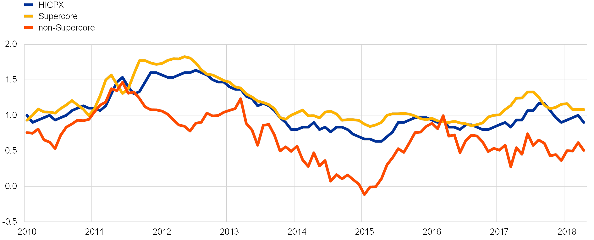
Sources: Eurostat and ECB calculations.
Notes: There are 47 HICP items in the latest vintage of Supercore. The latest observations are for April 2018.
Further along the spectrum of econometric complexity is another frequency-based measure referred to as the Persistent and Common Component of Inflation (PCCI), which filters out and averages the medium-term component of the HICP components of individual euro area countries. The PCCI captures the common and persistent component in inflation rates across countries and items (see Box 3). It is designed to signal developments in headline inflation, and in particular turning points, with some lead. As it also includes information on energy and food items, unlike some other measures of underlying inflation, it is important to assess to what extent changes in the PCCI are driven by energy and food components and to what extent they are driven by HICPX components. The PCCI, being based on a rather complex econometric model with many layers of filtering and averaging, presents challenges in interpretation. These are compensated for by the fact that it can be especially useful when several idiosyncratic shocks across countries and items also affect items that are normally not volatile.
Box 3 The Persistent and Common Component of Inflation (PCCI) measure of underlying inflation
The PCCI is a frequency exclusion measure of underlying inflation that uses time-series smoothing and exploits cross-sectional information across items and countries. It is designed to capture the persistent and common component of inflation rates across euro area countries and sub-items. The common component is estimated with a generalised dynamic factor model, in line with what has been previously proposed in the literature for the euro area[20] and also for a similar indicator for the United States.[21]
The indicator is constructed as follows: around 1,000 HICP sub-items from 12 euro area countries are collected and are seasonally adjusted, expressed in terms of annualised month-on-month rates (calculated as log-differences) and standardised to have a mean of zero and a standard deviation of one. The low-frequency common component for each sub-item is estimated with the generalised dynamic factor model. This requires the choice of a set of parameters, in particular the number of dynamic factors, the number of static factors and the threshold for the minimum length of cycles allowed in the common component. The PCCI excludes all cycles with a length shorter than three years.[22] In order to reduce the uncertainty about the number of factors, the common component for each sub-item is an average of 81 estimates obtained for different combinations of dynamic (from two to eight) and static (from four to 16) factors. The resulting low-frequency common components are resized using the mean and the standard deviation estimated in the first step and are smoothed with a three-month moving average.[23]
The PCCI is finally obtained by aggregating all the low-frequency common components using the weights of the single items in the total HICP. A similar aggregate, which is referred to as PCCIx, can be obtained for a sub-component, such as the HICP excluding energy and food, by aggregating only items which are part of this sub-component, or other aggregates can be calculated for any combination of sub-components and countries.
The main advantage compared with exclusion measures, such as HICPX, is that the PCCI also includes the impact of medium-term shocks affecting food and energy, to the extent that they have common effects, and, at the same time, it excludes short-term fluctuations in prices that are considered as “core” in the traditional exclusion measures (such as services prices). In general, the PCCI is a flexible indicator whose estimates depend on the set of variables included and the threshold of the highest frequency allowed, so that a practitioner may decide to reduce the persistence of the indicator by reducing the threshold to cycles with a length of more than one year, or to exclude food and energy shocks.
Chart A shows the PCCI estimate of underlying inflation for headline HICP inflation as described above, together with headline annual inflation and the measure of trend inflation defined as the centred moving average with a length of two years as proposed in Section 3. Compared with both measures, the PCCI is less volatile and less affected by large temporary shocks, such as the ones affecting energy prices that explain the negative inflation rates registered in 2009, 2015 and 2016. Chart B shows the same indicator obtained by aggregating only the common persistent components of items which are included in the HICPX index, i.e. excluding energy and food items. Naturally, this narrower PCCIx index is also less volatile and less affected by short-term movements than HICPX. In both cases, the PCCI indicators can anticipate peaks of annual inflation, but with a lag compared with the centred two-year moving averages. However, when considering how policymakers would look at underlying inflation indicators, it is important to consider that centred moving averages are not available in real time, as they use observations from the future.
Chart A
Headline inflation and the PCCI for headline HICP inflation
(annual percentage changes)

Sources: Eurostat and ECB calculations.
Note: The latest observations are for April 2018.
Chart B
HICPX and PCCIx for items included in the HICPX index
(annual percentage changes)

Sources: Eurostat and ECB calculations.
Note: The latest observations are for April 2018.
3 Empirical evaluation of the measures of underlying inflation
An empirical assessment can help to discriminate between the different measures of underlying inflation. Measures of underlying inflation should track the evolution of medium-term headline inflation. While this implies a challenge, as one wants to track an unobservable quantity, an assessment of the properties of the measures can be conducted based on a number of empirical criteria. These include volatility, coincidence, unbiasedness and overall precision.[24] Also, as the relative performance of a measure may be episodic, it is important to assess the measures over different periods of time.
An estimate of the persistent component of inflation is needed to assess the measures of underlying inflation. Trend inflation is an unobservable variable and its estimation is surrounded by high uncertainty. As a very rough proxy for trend inflation, this article uses a 24‑month centred moving average of monthly inflation, which should be sufficiently long to smooth out high-frequency fluctuations, yet short enough to reflect the horizon at which monetary policy operates over the business cycle.[25] Given that constructing this measure requires the use of future values of inflation, it has limited conjunctural use, but it can serve as a benchmark to assess other indicators.
Most measures of underlying inflation successfully filter out the volatility in headline inflation. The standard deviation, a crude measure of volatility, is generally significantly lower for the measures of underlying inflation than for the headline HICP inflation rate. The HICPX, HICPX excluding travel-related items, clothing and footwear, PCCI and Supercore measures tend to have comparatively low volatility (see Table 1). However, there is a trade-off between volatility and information content: for example, an index that is constant over time would have no volatility but would not capture any dynamics in trend inflation. This trade-off highlights why the assessment must be based on a set of criteria rather than on one criterion in isolation.
Table 1
Standard deviations of measures of underlying inflation

Sources: Eurostat and ECB calculations.
Yet, measures of underlying inflation still exhibit volatility, making it challenging to determine whether a cyclical turning point has occurred. One way to investigate this more formally is to apply a measure typically used for assessing the business cycle, the “months for cyclical dominance” (MCD) measure. The MCD measure gives the number of months it takes on average for the signal from the cyclical component of a series to dominate the noise of the series (for the construction of the MCD measure, see the notes to Chart 6). Looking at the MCD for the underlying inflation measures that do not already explicitly embed a filter, the HICPX tends to be noisier and can take relatively longer before the cyclical signal dominates (see Chart 6).
Chart 6
Noise-to-signal ratios for the measures of underlying inflation
(x-axis: number of months; y-axis: ratio of the volatility of changes in the irregular component to the volatility of changes in the cyclical component)

Sources: Eurostat and ECB calculations.
Notes: The PCCI is not included as it already explicitly embeds a filter. The construction of the MCD measure involves several steps. For each measure of underlying inflation, the cyclical and error (noise) components of the year-on-year rates of inflation are first estimated using a fixed-length symmetric Baxter-King band-pass filter. Then, the following are calculated across lags of one to 12 months: (i) the standard deviation of the changes in the cyclical component (this should increase, the longer the lag); and (ii) the standard deviation of the changes in the irregular component (this should be broadly the same across lags). The MCD is the monthly lag for which the ratio of (ii) to (i) begins to be substantially lower than one (the threshold is set at 0.7). It can then be said that the change in the series between month t and month t‑MCD would normally be in large part due to a cyclical movement. If the value of the measure of underlying inflation in month t is higher (lower) than its value in month t‑MCD, this suggests an upswing (downswing). In general, the smoother the series in its raw form, the lower the MCD tends to be. Based on a sample from January 2000 (March 2003 for Supercore) to April 2018.
The measures of underlying inflation are biased to varying degrees, suggesting that none of the measures is entirely successful in isolating the more permanent component. The measures of underlying inflation should demonstrate a close coherence with the in-sample persistent component of the HICP inflation trend.[26] If a measure does not capture well the latter, then its long-term average may diverge from that of headline inflation. The standard core measures (e.g. HICPX) tend to have a negative bias (pointing to lower than realised inflation over the whole period), partly reflecting that energy inflation has been relatively high on average over the sample period (see Table 2). In contrast, the more model-based measures (e.g. the PCCI and Supercore) tend to have a positive bias. In the case of Supercore, this may reflect that services items, which tend to have a higher inflation rate on average over time than non-energy industrial goods items, are more often selected as they tend to have a stronger link with the domestic business cycle. The bias of the trimmed means is relatively small over the full sample.
Table 2
In-sample accuracy of measures of underlying inflation
(percentage points)

Sources: Eurostat and ECB calculations.
Notes: The RMSE is computed by evaluating the error incurred by each of the different measures at each specific time t to capture the inflation trend at time t. All measures of underlying inflation are computed in “real time”, i.e. by considering only the information that would be available to the forecaster at time t. For example, in the case of Supercore, real-time vintages of the output gap are used.
The performance of the measures of underlying inflation in tracking the persistent component of headline inflation is episodic. The root mean squared error (RMSE) can be decomposed into two components, one due to the bias and another due to the ability of an index to track the month-on-month dynamics in the target variable. Over the full sample, the PCCI and the trimmed means tend to perform best in tracking the benchmark two‑year moving average of inflation. In the case of the trimmed means, this partly reflects their relatively low bias. Notably, HICP inflation excluding energy and food performs relatively poorly. However, over the more recent period, the measures of underlying inflation generally have a broadly similar performance, with the exception of Supercore, which tends to have a somewhat higher RMSE.
Measures of underlying inflation tend to lag the benchmark. Coincidence, which is measured by the correlation of headline inflation and the measures of underlying inflation at various leads and lags with the two-year centred moving average of monthly inflation, can help to assess whether the measures provide a timely signal about inflationary pressure. Generally, the measures exhibit a lagging behaviour with respect to the benchmark (see Charts 7 and 8), which suggests that it may be challenging for these measures to accurately track the future development of the inflation trend. This can also be gauged with a more formal analysis of the out-of-sample predictive ability of the different measures.
Chart 7
Correlations of permanent exclusion measures with the two-year moving average of HICP inflation at 12 leads and lags
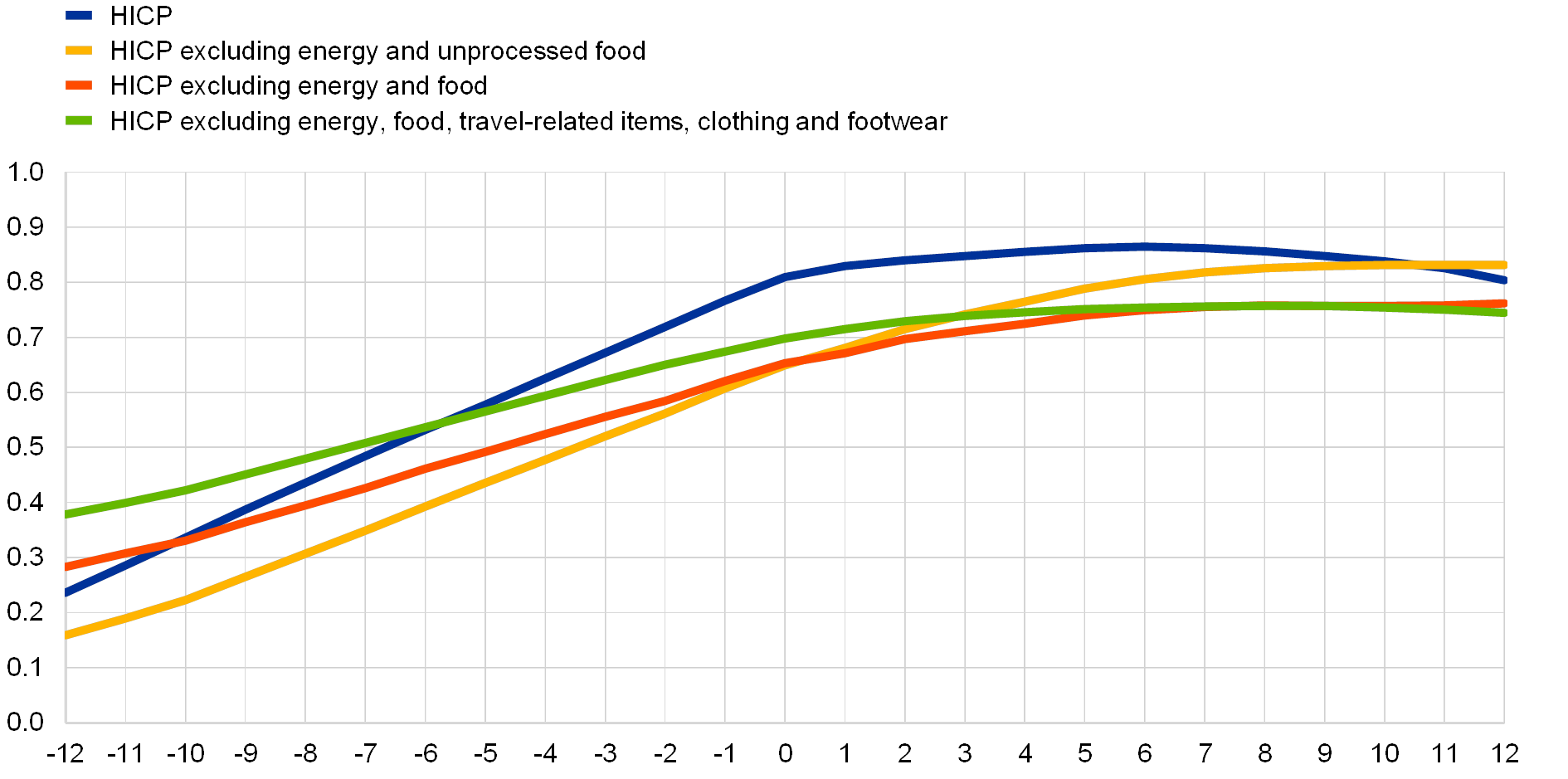
Sources: Eurostat and ECB calculations.
Notes: The sample period is January 2000 to April 2018. The x-axis indicates the number of lags for the permanent exclusion measures of underlying inflation, while the y-axis shows their correlation with the two-year centred moving average.
Chart 8
Correlations of temporary and frequency exclusion measures with the two-year moving average of HICP inflation at 12 leads and lags

Sources: Eurostat and ECB calculations.
Notes: The sample period is January 2000 to April 2018. The Supercore measure is not included as vintages only begin in 2007. The x-axis indicates the number of lags for the temporary or frequency exclusion measures of underlying inflation, while the y-axis shows their correlation with the two-year centred moving average.
The predictive accuracy of the measures of underlying inflation varies strongly over time (see Table 3). The out-of-sample ability of the measures of underlying inflation to track the future development of the benchmark varies over the assessment sample.[27] According to statistical tests, the bias is not significantly different from zero[28] for any of the measures over the full sample or the shorter sample.[29] Concerning more generally the significance of the differences in forecast accuracy across different measures, the HICP excluding energy and food is taken as a benchmark. While in the full sample the differences across measures turn out to be insignificant, in the shorter sample the trimmed means and the Supercore perform significantly worse than the HICPX.[30] However, it should be stressed that the relative performances of all measures tend to vary considerably over different sub-samples, suggesting that a range of measures should be monitored. It is also worth noting that combining all the measures into one composite index is not likely to be a much better solution to analysing the range; for example, all the measures of underlying inflation show a positive bias over the past decade which is even magnified in the more recent part of the decade, suggesting that an average of many measures would not have a much better performance.
Table 3
Out-of-sample accuracy of measures of underlying inflation
(percentage points)

Sources: Eurostat and ECB calculations.
Notes: All measures of underlying inflation are computed in “real time”, i.e. by considering only the information that would be available to the forecaster at time t. See also the notes to Table 2. For example, in the case of Supercore, real-time vintages of the output gap are used.
Measures of underlying inflation should also satisfy some practical criteria. Firstly, they should be available on a timely basis. Some of the measures (e.g. the HICP excluding energy, food, travel-related items, clothing and footwear, the PCCI and Supercore) can only be constructed when the full release of monthly data is available, which is generally about two weeks after the flash release. Also, the measures should ideally not be subject to data revision. Most of the measures are not revised but there are some notable exceptions. In particular, the PCCI series can be revised because the seasonal adjustment of the underlying data produces revisions over the whole sample with the introduction of each new observation. The Supercore series is revised not only as the seasonally adjusted series change, but also on account of the output gap series being revised over time (often quite substantially) and of the shifting out-of-sample forecast horizon.
It is also helpful if the measures of underlying inflation are sufficiently transparent that they can be easily communicated to the public. Developments in permanent exclusion measures can be easier to communicate as any divergence from headline inflation can be attributed to certain sub-components (e.g. energy). It can be somewhat more challenging in the case of temporary exclusion measures as, at any given point in time, it may be necessary to identify which items are excluded and explain if and how their outlying behaviour reflects the influence of temporary phenomena. The Supercore and the PCCI measures are based on statistical methodologies, which poses more communication challenges. Also, the results can sometimes be challenging to interpret. Overall, while some measures may have performed relatively well in tracking the benchmark inflation (e.g. the PCCI over certain periods), they may come with the downside of being more challenging to explain to the public.
Overall, there is no single measure that emerges as optimal across all criteria. The relative performance of the measures tends to be episodic. As individually the measures may not consistently give very precise or reliable signals, this calls for monitoring a wide range of measures of underlying inflation.
4 Conclusions
Measures of underlying inflation offer different perspectives and insights that together can be helpful in understanding developments in headline inflation. Tracking developments in HICPX is useful during periods when there are large and temporary swings in energy and food prices. HICPX excluding travel-related items, clothing and footwear becomes very relevant when calendar effects are prominent. Indicators that exclude outliers can also at times play a useful complementary role. The Supercore indicator goes further by excluding those items that are estimated to be insensitive to domestic real economic conditions. Still, every item in the HICP is driven to some extent by permanent factors, albeit to a relatively small degree in some cases, and these items can contain useful information about underlying inflationary pressure. The PCCI dynamic factor model tries to exploit this by capturing the persistent component across all items of the HICP and across several euro area countries.
Empirical results suggest that no one measure of underlying inflation is superior in all situations as the performance of the indicators varies over time. In practice, each indicator comes with merits and shortcomings, which calls for monitoring the full range of measures of underlying inflation. Generally, measures of underlying inflation are only a first pass at quantifying underlying inflationary pressure over the medium term. They need to be complemented by a more structural examination of the driving forces in order to better understand the inflation process.
- In what follows, the persistent component of inflation is simply defined as “trend inflation”, although different concepts of trend inflation exist. For example, over the longer term, trend inflation can be seen as reflecting the quantitative inflation objective and the credibility of the central bank in achieving it.
- For recent evidence on the drivers of inflation, see for example the article entitled “Domestic and global drivers of inflation in the euro area”, Economic Bulletin, Issue 4, ECB, 2017.
- In September 2017 Sveriges Riksbank adopted the CPIF as its inflation target variable. The CPIF is based on the CPI, but excludes the effects of changes to mortgage rates. The change was motivated by the fact that household mortgage costs change in lockstep with the official interest rate and therefore their inclusion in the CPI caused a part of the inflation target measure to be positively correlated with the policy instrument. Indeed, Sveriges Riksbank had been using the CPIF as a de facto operational target variable for several years before it became the formal target variable for monetary policy.
- See Monetary Policy Report, Federal Reserve Board, July 2017.
- See “Performance of Core Indicators of Japan’s Consumer Price Index”, Bank of Japan Review, 2015-E-7.
- See the May 2017 and August 2017 Bank of England Inflation Reports.
- See Renewal of the inflation-control target: Background information, Bank of Canada, October 2017.
- See also Box 1 on measures of underlying inflation used at selected central banks.
- Travel-related items comprise air fares, package holidays and accommodation services.
- Changes in indirect taxes or administered prices tend to be one-off effects that have little relevance for medium-term inflation. To this end, measures of inflation that exclude indirect taxes and/or administered prices are also assessed, although not on a routine basis. See, for example, the box entitled “Measuring and assessing the impact of administered prices on HICP inflation”, Monthly Bulletin, ECB, May 2007.
- HICPX excluding travel-related items, clothing and footwear accounts for about 60% of the HICP basket, while HICPX accounts for about 71% of the HICP basket.
- For an illustration of why high volatility may not always be associated with low persistence, see also Bilke, L. and Stracca, L., “A persistence weighted measure of core inflation in the euro area”, Economic Modelling, Vol. 24, 2007, pp. 1031‑1047.
- The analysis is based on annual inflation rates. The ordering of the sub-components in terms of both volatility and persistence remains broadly similar when seasonally adjusted month-on-month inflation rates are examined.
- It is worth keeping in mind that the persistence of services inflation is higher than that of individual series partly because the aggregation can help to wash out idiosyncratic effects.
- For more background, see Glossary: COICOP HICP on the Eurostat website.
- The 10% (30%) trimmed mean removes 5% (15%) of the annual rates of change from each tail of the distribution of 93 price changes in the HICP each month and aggregates the annual rates of change using rescaled weights. The (weighted) median is an extreme form of the trimmed mean as it trims all but the (weight-based) mid-point of the distribution of price changes. See also Silver, M., “Core inflation: Measurement and statistical issues in choosing among alternative measures”, 2007.
- See also the box entitled “The role of seasonality and outliers in HICP inflation excluding food and energy”, Economic Bulletin, Issue 2, ECB, 2018.
- Notice that the Supercore measure could also be classified as a temporary exclusion measure because, as opposed to excluding HICPX items a priori, it excludes some items on the basis that they are estimated not to be very related to domestic business cycle fluctuations. However, it is better understood as a frequency exclusion measure as, among HICPX items, it picks out those that are more correlated with the business cycle.
- See the box entitled “The responsiveness of HICP items to changes in economic slack”, Monthly Bulletin, ECB, September 2014. This was an earlier version of Supercore that selected HICPX items for inclusion if the coefficient of the output gap had an economically meaningful sign and a statistically significant coefficient in a Phillips curve equation. This approach is more straightforward to implement, but may suffer from omitted variable bias and tends to select relatively few items. An equation similar to the one presented in the above-mentioned box was previously estimated by the Deutsche Bundesbank for the same purpose: see Fröhling and Lommatzsch, “Output sensitivity of inflation in the euro area: indirect evidence from disaggregated consumer prices”, Discussion Paper Series 1: Economic Studies, No 25, Deutsche Bundesbank, 2011.
- Cristadoro, R., Forni, M., Reichlin, L. and Veronese, G., “A core inflation indicator for the euro area’’, Journal of Money, Credit and Banking, Vol. 37, 2005, pp. 539‑560. The PCCI differs from this core inflation indicator because it excludes cycles with a length shorter than three years, while the above-cited article excluded only cycles with a length of one year. The set of variables used for the estimation only includes HICP sub-items and the average of the estimates obtained using different numbers of static and dynamic factors is used. For an application of this methodology to aggregate euro area data, see Lenza, M., “Revisiting the information content of core inflation”, Research Bulletin, Vol. 14, ECB, 2011, pp. 11‑13.
- “The FRBNY Staff Underlying Inflation Gauge: UIG”, Federal Reserve Bank of New York Staff Report No 672, April 2014.
- The profile of the PCCI is also similar when excluding only cycles with a length shorter than two years.
- As explained for Supercore, this final step helps to lessen the chances of a false positive signal when assessing turning points.
- See, for example, the box entitled “Are sub-indices of the HICP measures of underlying inflation?”, Monthly Bulletin, ECB, December 2013.
- All the results presented in this section are qualitatively robust to the adoption of a 36‑month moving average.
- In this exercise, the proxy for trend inflation is defined as the annualised moving average of HICP inflation for two years centred at time t, i.e. it is equal to 1,200*(pt+h – pt-h )/(2*h) where h is 12 months.
- The trend inflation target in month t is defined as the annualised HICP growth rate over the subsequent two years, i.e. it is equal to 1,200*(pt+H – pt )/H where H is 24 months.
- For all the tests carried out in this section, 5% is the level considered to gauge statistical significance.
- The significance of the bias terms is assessed by means of a t-test with heteroskedasticity and autocorrelation consistent standard errors.
- A Diebold-Mariano test, again accounting for heteroskedasticity and autocorrelation consistent standard errors, is used to determine whether one measure performed statistically better than the HICP excluding energy and food.