
Economic shocks and contagion in the euro area banking sector: a new micro-structural approach
Economic shocks and contagion in the euro area banking sector: a new micro-structural approach
Published as part of the Financial Stability Review May 2019.
The financial system can become more vulnerable to systemic banking crises as the potential for contagion across financial institutions increases. This contagion risk could arise because of shifts in the interlinkages between financial institutions, including the volume and complexity of contracts between them, and because of shifts in the economic risks to which they are commonly exposed. Analysis of the euro area banking system’s interlinkages, using the newly available large exposure data, suggests that the system could be more vulnerable to financial contagion through long-term interbank exposures than noted in other studies. That said, common exposures to the real economy – a standard contagion channel in the literature – represent a potential source of individual bank distress and non-systemic events. This analysis also provides an insight into the changes in contagion risk in the system over time, helping us to interpret changes in market indicators of systemic risk, such as aggregated credit default swap (CDS) prices.
1 Introduction
Contagion – or the phenomenon of a negative shock (or bad news) spreading rapidly across the financial system – is a feature of nearly all systemic banking crises. The many interconnections between different financial institutions, households and businesses allow the financial system to work efficiently in good times, but they can also make the system more vulnerable to bad events being transmitted rapidly across institutions and amplified into systemic events. These events generally involve multiple banks failing at the same time.
The financial system can become more vulnerable to systemic banking crises as the potential for contagion increases. Broadly speaking, there are two ways in which contagion risk is thought to arise: interconnections and common exposures. Interconnections are the direct linkages between households, businesses and financial institutions – such as loans, collateral arrangements and derivatives contracts. These linkages allow financial agents to transfer risk among each other, supporting capital allocation in normal conditions. But they can also transmit problems from one institution to others in stressed conditions. Common exposures, for example when many institutions have similar portfolios of securities or loans, will reflect the underlying demand of the economy for financial intermediation. However, if one or more institutions face losses on their portfolios, or start fire-selling assets to manage other problems, then institutions with similar portfolios may also see values deteriorate.[2]
Post-crisis reforms to financial regulation include measures to try to mitigate the risk of contagion. These measures include the introduction of the large exposure regime, which limits the extent to which a bank can be exposed to a single entity, additional capital requirements for systemically important institutions, the new regulatory liquidity ratios and changes to the requirements for margining derivatives contracts. Central bank lending facilities should also support core market functioning in a stress episode, limiting the risk of fire sales.
This special feature uses newly available granular data on euro area banking sector exposures, combined with a micro-structural model, to examine the potential for contagion in the euro area financial system. In recent years, a number of papers have set out models of the behaviour of individual agents reacting to different types of shocks, and the interactions between these agents, aimed at reproducing the complex dynamics of a financial crisis. These models usually rely heavily on very granular data on banks’ exposures, which are difficult to obtain outside the regulatory environment.[3] In this special feature, we combine a model of this type with multiple sources of granular information on the exposures of euro area banks. This includes the recently available time series of data captured as part of the regulation to limit banks’ losses in relation to a single entity, or large exposure data. These data are then used to assess the probability of a banking crisis (i.e. multiple banks failing at the same time) as a result of risk propagation either due to systematic risk that stems from common exposures to real sectors vulnerable to similar economic risk or through one of three contagion channels: (i) long-term interbank exposures vulnerable to financial credit risk due to counterparty default; (ii) short-term interbank exposures vulnerable to liquidity shocks; and (iii) common securities holdings vulnerable to market risk in the event of fire sales.
2 Data on exposures
Analysing how losses could spread through the financial system in a crisis, from a bottom-up or micro-structural perspective, requires detailed information about euro area banks’ exposures to households, businesses, as well as other banks and financial institutions. The large exposure regime, introduced in the EU in 2014, limits the maximum loss a bank could incur in the event of a sudden counterparty failure, and requires banks to report to prudential authorities detailed information about their largest exposures. An exposure to a single client or connected group of clients is considered a large exposure when, before applying credit risk mitigation measures and exemptions, it is 10% or more of an institution’s eligible capital (Article 392 of the Capital Requirements Regulation). Moreover, institutions are also required to report large exposure information for exposures with a value above or equal to €300 million. Therefore, the data reported capture almost €8.2 trillion of gross exposures in the third quarter of 2018 (our reference date), i.e. more than 50% of euro area credit institutions’ exposures. These data can be organised and mapped with statistical techniques to arrive at a unified identifier for each of the parties involved in almost any exposure. The data processing eventually provides exposure-level information about the euro area banking system’s exposures to entities worldwide, covering all economic sectors: credit institutions, financial corporations, non-financial corporations, general government and households.
Chart B.1 compares the large exposure (LE) coverage of euro area significant institutions (SIs) with total assets by sector. As we can see, large exposures to credit institutions, financial corporations and governments account for 77%, 67% and 98% respectively of euro area SIs’ total assets vis-à-vis these sectors. The coverage of non-financial corporations is lower, at approximately 31% of SIs’ total assets, whereas the household sector is barely covered. In this special feature, we focus primarily on the exposures to other credit institutions, i.e. the interbank network of large exposures. The extensive coverage of this sector in the LE data provides us with confidence that we can reliably model euro area banks’ degree of interconnectedness and their contribution to cross-sectional systemic risk. Where needed, the LE dataset is complemented with LE data reported by euro area less significant institutions (LSIs), and with additional information concerning exposures of euro area SIs to euro area LSIs and of non-euro area banks to euro area SIs and LSIs from COREP template C.67 reporting the ten largest euro area banks’ liabilities.
The large exposure dataset is significant
Euro area significant institutions’ large exposure coverage across sectors and total assets
(€ trillions)

Sources: ECB supervisory data and ECB calculations.Note: CI stands for credit institutions, FC for financial corporations, NFC for non-financial corporations, GOV for general government and HH for households.
Table B.1 sets out what the combined data indicate about interbank exposures in the euro area, while Chart B.2 shows the interlinkages identified between euro area banks. In the third quarter of 2018 more than one thousand banks were covered by these data, with around €2.3 trillion of gross exposures between them, of which roughly 60% has a maturity below 30 days. The interbank network has a density of links just above 0.4%, implying that the level of interconnectedness is relatively low and markets are segmented. Furthermore, the degree distribution of the network is well fitted by a power law with an exponent of 1.35, meaning that there are a few banks playing a central role in the system, while most of the institutions are peripheral. This structure mirrors findings already established in the literature about financial networks.[4]
Interbank network
(amounts in € trillions)
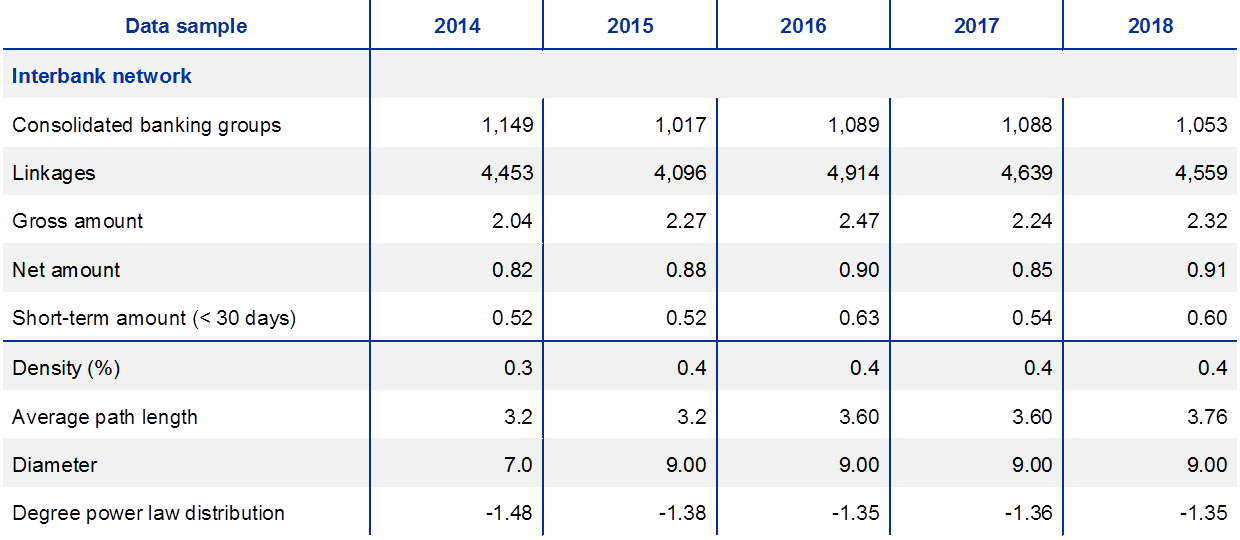
Source: ECB supervisory data and ECB calculations.Notes: Consolidated banking groups refer to euro area and non-euro area banks. Net amount is the amount of unsecured exposures, and refers to the gross amount after deducting exemptions and credit risk mitigation.
Interconnectedness is relatively low and markets are segmented in the euro area interbank network
Euro area interbank network of large exposures
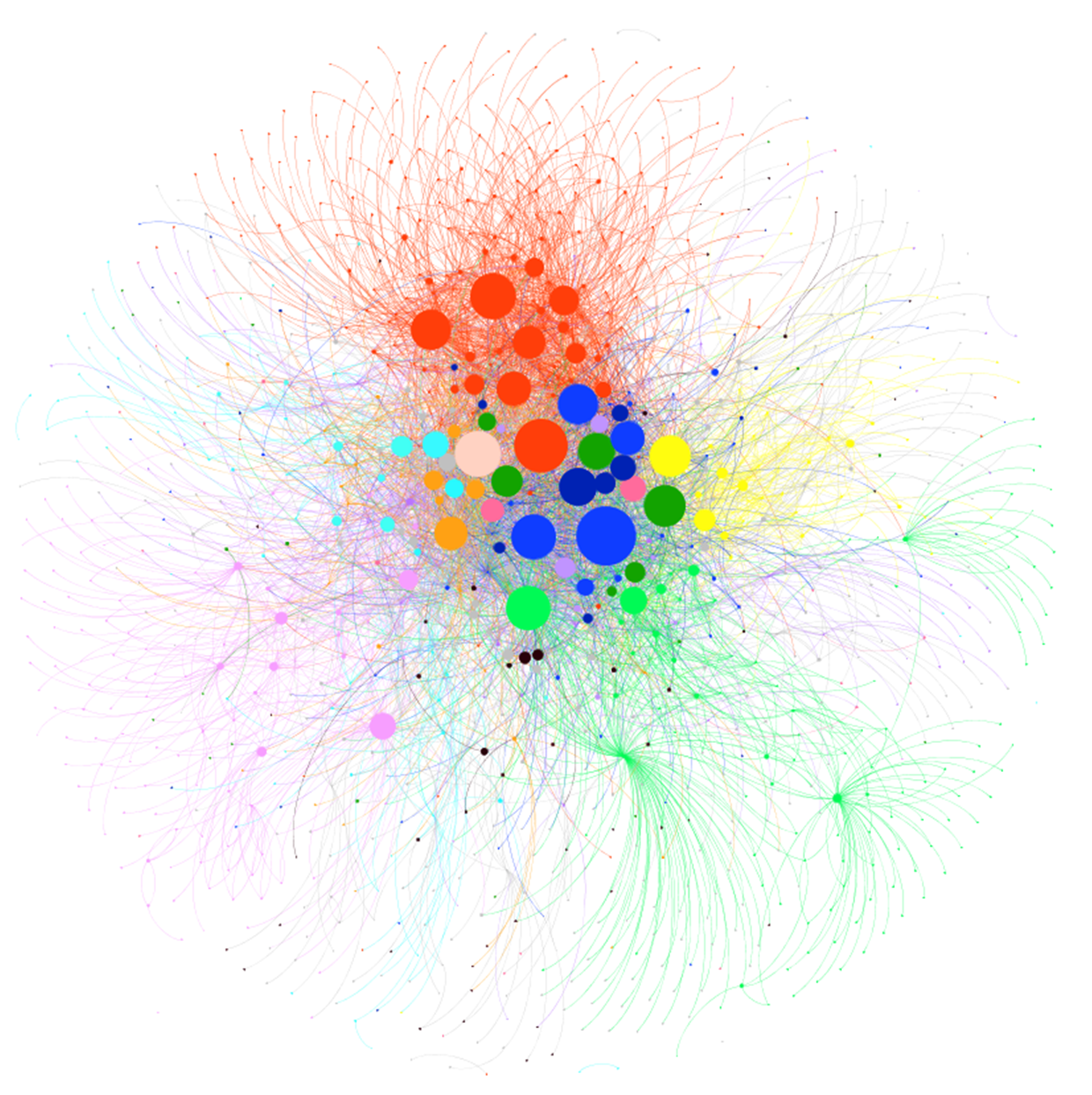
Sources: ECB supervisory data and ECB calculations.Notes: The node size captures the weighted in-degree of interconnectedness. The node colour represents the country of origin. The thickness of the links reflects the value of the exposures in € billions. The colour of the links refers to the country of the target, thus also capturing the borrower’s perspective.
3 Modelling systemic events
This special feature uses simulations to examine how different contagion channels might lead to a systemic crisis, using recent real data. We do this by estimating the range of losses that banks could face on their portfolios, using information on probabilities of default (PDs), loss given default (LGD) and correlation among their portfolios of exposures to the real economy. The losses generated by common real exposures account for only a part of the final correlation in banks’ distress probabilities observed in reality, providing a first contribution to the number of defaults determining a systemic event. On top of that, other financial contagion channels further exacerbate common distress among banks. This special feature aims to disentangle the different contributions to systemic risk.
As shown in Figure B.1, each simulation follows the same chain of events, as follows:
- Realisation of economic risk. Each individual bank is faced with losses on its loan portfolios in line with the performance of households and non-financial corporations in that simulation. To generate these losses, each real economy entity is assigned a PD, an exposure-specific LGD, and a correlation structure of PDs retrieved, respectively, from Moody’s, the LE dataset and Datastream.[5] This may lead some banks to default.
- Spread and realisation of interbank financial credit risk. Any defaulted bank then transmits losses to its counterparties through the long-term interbank market. Credit risk can therefore materialise, further eroding banks’ capital and causing other banks to either default or become distressed.
- Spread and realisation of liquidity risk. Defaulted and distressed banks withdraw liquidity from the interbank market, as precautionary hoarding against future shocks. The short-term interbank market freeze generates liquidity risk, which can translate into capital erosion in the next step.[6]
- Spread and realisation of market risk. Illiquid banks may sell securities abruptly. Prices endogenously adjust via a fire-sale mechanism, and banks with mark-to-market exposures may see their capital further eroded. Market risk can therefore materialise.[7]
The sequence of events 2, 3 and 4 repeats itself until no additional default or distress event is experienced in the system. The simulation is repeated for 50,000 different initial economic losses in order to obtain a distribution of the number of distressed and defaulted banks.
System mechanics
The block scheme summarises how the various risk channels interact within the contagion model, while the chart depicts in a sequential order the trigger event (scenario), the amplification mechanisms, and the final vector of bank defaults

Source: ECBNote: Economic risk captures initial losses derived from the scenario which is a function of entity-specific PDs, an exposure-specific LGD, and a correlation structure of default probabilities .
4 Identification of systemic events
A systemic banking crisis is characterised by a sharp rise and persistence in the number of distressed and defaulted banks. Chart B.3 shows the pattern of bank distress and default (blue line) in the United States and in the European Union, and the association with severe economic crises (dark grey areas) relative to milder economic downturns (light grey areas). The series suggest that the financial industry might be a two-state system, where either there are no distressed banks at all, or many banks run into trouble at the same time. This stylised fact is consistent with the observation that market-based estimates of bank distress probability are highly correlated. Furthermore, when the number of distressed and defaulted banks in a quarter rises above a certain threshold (x) close to 1.5%, it tends to remain so for many quarters.[8]
Hence, an increase in the share of banks in distress or default (D) to above 1.5% at a point in time (e.g. a quarter) can be used as a simple yardstick of financial (in)stability.
Interconnectedness is relatively low and markets are segmented in the euro area interbank network
Fraction of distressed and defaulted banks in the United States (left panel) and in Europe (right panel)
(percentages)
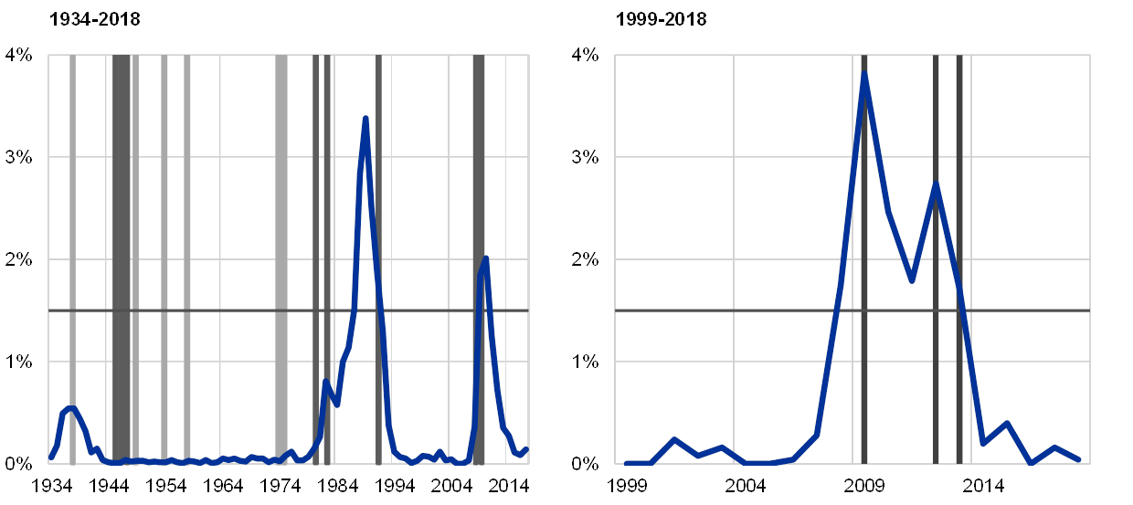
Sources: Lang et al. (2018) for the European bank distress time series, and Federal Deposit Insurance Corporation for the US time series.Notes: Bank distress is defined as one of the following events: (i) capital injection; (ii) asset protection scheme; (iii) guarantee loan; (iv) state aid; or (v) bankruptcy. Light grey and dark grey areas represent mild and deep economic recession periods, respectively. Mild economic recessions refer to periods during which real GDP experienced negative growth rates, while deep economic recessions refer to periods during which real GDP experienced growth rates lower than -1%.
5 Results
The simulation results can be used to estimate the probability that the share of banks in distress could be above this threshold, based on their current balance sheet composition. Table B.2 reports the probability of a systemic event arising in the third quarter of 2018 and the distribution of the number of defaults for each source of risk for the third quarter of 2018, respectively and in combination: (i) economic risk; (ii) economic risk and market risk; (iii) economic risk and liquidity risk; (iv) economic risk and financial credit risk; and (v) when all the channels are simultaneously active, that is total risk.
Long-term credit interlinkages between banks triple the likelihood of a systemic event, while common exposures to the real economy seem to be the second most important determinant of systemic events. The interaction of economic risk from common exposures with the other contagion channels increases the probability of a systemic event non-linearly. For instance, when economic risk interacts with financial credit risk derived from long-term interbank exposures, the probability of experiencing a systemic event triples (to 0.196%), whereas all the channels taken together produce a number of systemic events four times larger than economic risk alone, with an associated probability of 0.224%.
Financial amplification mechanisms appear sizeable in the euro area financial system, and could make a significant contribution to the probability of experiencing a systemic event. Moreover, as shown in Table B.2, a consistent share of the total number of defaults across all scenarios, almost 11%, is explained by the tail of the distribution, that is, by the realisation of systemic events. Interaction among contagion channels accounts for approximately 1.5% of total defaults in the tail of the distribution. Notably, the average probability of an individual bank default seems to be most affected by economic risk, and the other contagion channels only slightly affect the mean of the distribution.
Summary statistics of the results for the third quarter of 2018

Sources: ECB supervisory data and ECB calculations.Note: The interaction term is approximated by the difference between each contagion channel and economic risk, thereby providing a conservative estimate of amplification effects.
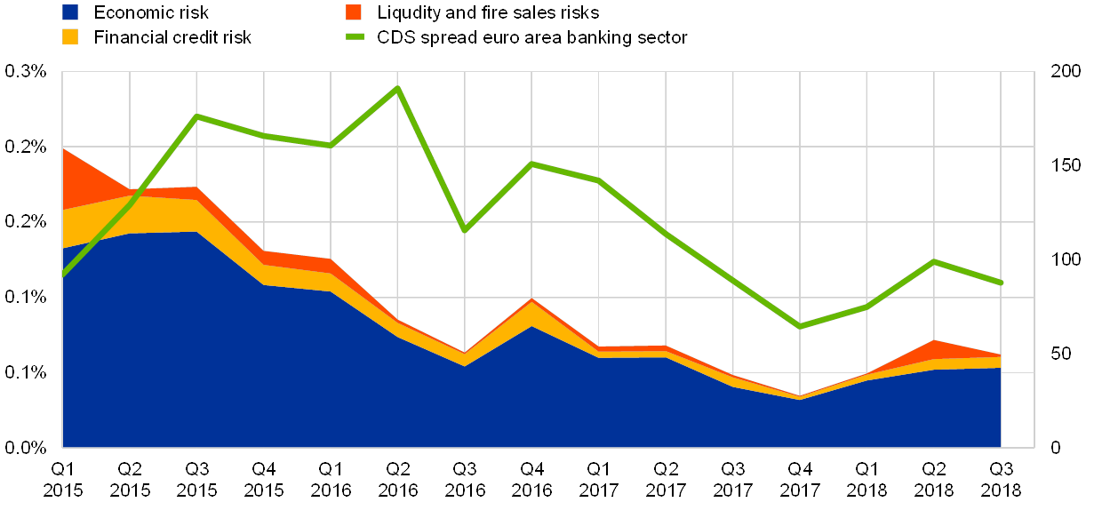
Charts B.4 and B.5 show the evolution since 2015 of the estimated probability of a systemic event, and of the average probability of an individual bank being in distress. Over the whole period, contagion and amplification mechanisms contribute more than economic risk to total systemic risk. In contrast, economic risk is the main driver of the mean of the distribution, i.e. the average probability of a bank default. There is also some indication of a decline in systemic risks coming from interconnectedness over the past four years. The trend of the systemic risk measure proposed in this special feature resembles the bank CDS index over the same time period, suggesting consistency between the estimation of banks’ joint PD and the probability of a systemic event.
Systemic risk over time
Probability of a systemic event, i.e. having more than 1.5% of banks in distress in the same quarter
(percentage probability (left-hand scale); CDS spread in basis points (right-hand scale))
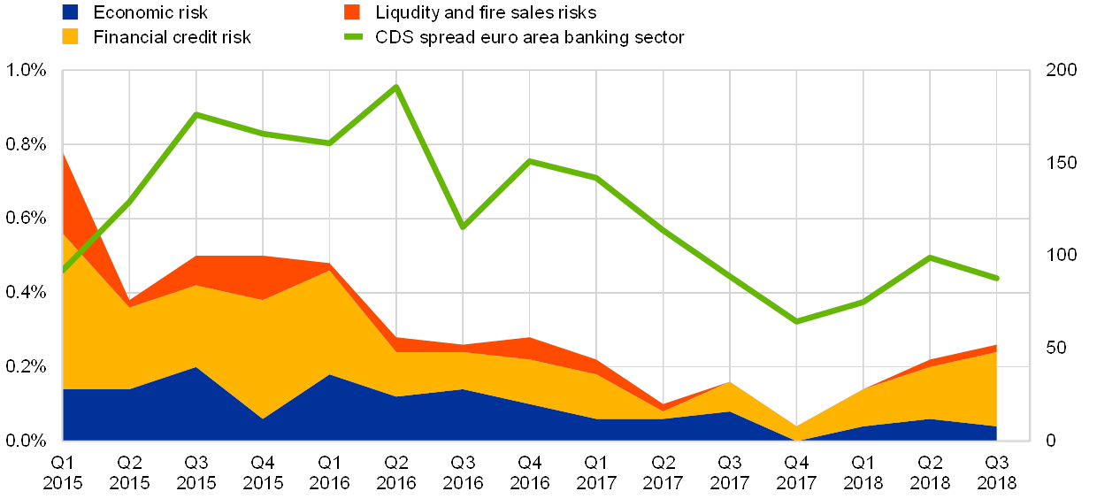
Sources: Thomson Reuters Datastream, ECB supervisory data and ECB calculations.Notes: The total probability of a systemic event is decomposed for each quarter into: (i) economic risk, i.e. the fraction of the total probability that is due to common exposures to the real economy; and (ii) financial risk, i.e. the fraction of the probability that is due to financial contagion, divided into interbank credit risk and liquidity and fire-sale risk. The CDS spread for the euro area banking sector is also plotted as a comparator.
Average probability of default of a bank over time
Average probability of default of a bank (probability of a single bank failing averaged over the entire sample, per quarter)
(percentage probability (left-hand scale); CDS spread in basis points (right-hand scale))
Sources: Thomson Reuters Datastream, ECB supervisory data and ECB calculations.Notes: The average probability of default of a bank is decomposed for each quarter into: (i) economic risk, i.e. the fraction of the total probability that is due to common exposures to the real economy; and (ii) financial risk, i.e. the fraction of the probability that is due to financial contagion, divided into interbank credit risk and liquidity and fire-sale risks. The CDS spread for the euro area banking sector is also plotted as a comparator.
6 Conclusion
This special feature presents a measure of systemic risk, derived from contagion risk and common exposures in the euro area banking system. The model employed encompasses four contagion channels, and their interaction generates non-linear effects that cannot be captured by studying the single contagion channels in isolation. The results indicate some decline in systemic risks coming from interconnectedness over the past four years. The trend of the systemic risk measure proposed in this special feature resembles the bank CDS index over the same period. This is noteworthy, as the index in this special feature is built using granular data on banks’ exposures to the real economy and to each other.
Combining a micro-structural model with newly available granular data allows us to disentangle the contributions of different factors and institutions to systemic risk. Exposures to the real economy seem to make the most important contribution to average default probabilities in the euro area banking system, while long-term bilateral exposures among banks seem to play the most important role in systemic risk for a given economic shock. Importantly, the trend in systemic risk as measured in this special feature resembles that in market-based indicators. The advantage of micro-structural models lies in the possibility to disentangle the different components contributing to systemic risk, and to identify key players in each market segment. The same models can be used in a wide variety of exercises, and the simulation engine can be easily fine-tuned to track the effects of each institution on systemic risk, or to understand the impact of a particular macroprudential policy on the financial system.
Box A Methodology
The methodology employed is built upon the multilayer framework of Montagna and Kok (2016) and the CoMap methodology developed by Covi et al. (2019).The dynamics of the model work as follows.
The system is composed of N banks, M real economic agents and L securities. Each bank status is related to two main idiosyncratic characteristics relating to its balance sheet, namely its capital and its liquidity , where “i” labels the bank. A bank is considered to be in distress if, for any reason during the simulation dynamics, its capital breaches its capital buffer requirements or its liquidity breaches the liquidity coverage ratio. In the same fashion, a bank is considered to have defaulted if its capital goes below its minimum capital requirements or its cash reserves are exhausted. Real economic entities are instead characterised by a probability of default ( ), a loss given default ), and a correlation matrix C, expressing joint default probabilities among non-financial corporations. Finally, each security is characterised by an initial price . With the dynamics of the model unfolding, the price of the security “l” is affected by how much of its notional has been sold ( ), according to the linear endogenous price function .[9]
The simulations start with the generation of the economic shock, i.e. a vector D of Bernoulli variables containing the information on whether corporation j defaulted ( ) and therefore generated losses for its lenders, or alternatively the corporation performed well ( ). The vector D is drawn according to the and C, and the losses generated by this mechanism produce a certain number of distressed and defaulted banks ( ). At this point, there is already a certain probability of having a systemic event, that is:
We will refer to this amount as economic risk. The contagion following this initial economic shock evolves in discrete time steps. Each time step is characterised by the sequence of three main events. First of all, at the beginning of each time step defaulted banks transmit losses to their counterparties in the long-term interbank exposure segments. This capital erosion may increase the number of banks in default or in distress. In a second step, distressed and defaulted banks leave the interbank market. This is done by withdrawing all their short-term liquidity from their borrower banks. At the same time, they are supposed to close the short-term interbank positions and they may do so by using a cash buffer, characteristic of each bank’s balance sheet. If any bank continues to have unfulfilled liquidity, they enter the last time step. Finally, in this stage, banks sell securities according to their liquidity needs in order to pay back creditors, and prices adjust accordingly. Banks with mark-to-market portfolios may see their capital eroded by the reduction in the price of the securities.
At the end of each simulation, we count the total number of defaulted and distressed banks ( ). At this point, we are able to compute the total amount of systemic risk in the system, which is:
- [1]Comments from Marco D’Errico are acknowledged.
- [2]See, for example, Duarte, F. and Eisenbach, T. M., “Fire-Sale Spillovers and Systemic Risk”, Federal Reserve Bank of New York Staff Report, 2018; Shleifer, A. and Vishny, R. W., “Fire Sales in Finance and Macroeconomics”, NBER Working Paper No 16642, 2010; Cont, R. and Schaanning, E., “Fire Sales, Indirect Contagion and Systemic Stress Testing”, Norges Bank Working Paper No 2/2017, 2017.
- [3]For a review of the literature, see Glasserman, P. and Young, P., “Contagion in Financial Network”, Journal of Economic Literature, Vol. 54(3), 2016, pp. 779-831.
- [4]See, for example, Lux, T. and Fricke, D., “Core-periphery structure in the overnight money market: evidence from the e-MID trading platform”, Computational Economics, Vol. 45(3), 2015, pp. 359-395.
- [5]Exposures to households are modelled with aggregate data at country level since the LE dataset has very limited coverage of this sector. In this respect, in order to compute the euro area banks’ losses, we use the average PD and LGD of the sample. The same holds for non-financial corporations, for which no public data about PD and LGD are available. To build the correlation structure necessary to generate the initial economic shock, NFCs’ CDS prices are used over a time horizon of one year before the end of the quarter under study. If any information is missing, the sector-country average is used.
- [6]See Acharya, V. V. and Merrouche, O., “Precautionary Hoarding of Liquidity and Interbank Markets: Evidence from the Subprime Crisis”, Review of Finance, Vol. 17, 2012, pp. 107-160; Kapadia, S., Drehmann, M., Elliott, J. and Sterne, G., “Liquidity Risk, Cash Flow Constraints, and Systemic Feedbacks”, in Haubrich, J. G. and Lo, A. W. (eds.), Quantifying Systemic Risk, University of Chicago Press, 2013, pp. 29-61.
- [7]See Cont, R. and Schaanning, E., “Fire Sales, Indirect Contagion and Systemic Stress Testing”, Norges Bank Working Paper No 2/2017, 2017.
- [8]In our framework, we adopt a quantitative measure to assess the probability that a systemic event will happen. This threshold is included between the 90th and 95th percentiles of the distribution, thereby capturing extreme events. See Box A for a more formal description of this measure.
- [9]See Greenwood, R., Landier, A. and Thesmar, D., “Vulnerable Banks”, Journal of Financial Economics, Vol. 115(3), 2015, pp. 471-485.