
Monetary policy and inequality
Monetary policy and inequality
Published as part of the ECB Economic Bulletin, Issue 2/2021.
1 Introduction
The issue of economic inequality began to receive increased attention after the global financial crisis. During that period, the increase in unemployment, the heterogeneous evolution of house and stock prices, and the fall in interest rates all affected households in very different ways. Income and wealth inequality has risen in most advanced economies since the early 1980s, with some countries now seeing levels comparable to those recorded at the start of the 20th century, raising increasing concerns regarding the political and economic consequences of that trend.[1]
More recently, there has also been a greater focus on the interaction between monetary policy and inequality. In response to the global financial crisis, monetary policy embarked on a prolonged period of monetary accommodation, with unconventional measures (such as forward guidance and asset purchases) being used to lower and flatten the yield curve. As such measures tend to have a larger impact on the price of long-term assets than changes in short-term interest rates, this has given rise to concerns that monetary policy is mainly benefiting wealthier households.[2] In addition, given the growing recognition that the pass-through of monetary policy is dependent on the distribution of income and wealth, central banks have begun to pay more attention to the heterogeneity of households.[3] These developments have been supported by a wealth of new academic research on the role that household heterogeneity plays in the transmission of macroeconomic shocks and policies.[4]
This article reviews the latest evidence on economic inequality and its interaction with monetary policy, with a particular focus on the euro area. Section 2 analyses both secular trends and cyclical fluctuations in the distribution of income and wealth in the euro area (a distinction that matters, since the interaction between monetary policy and inequality is arguably fairly cyclical in nature). Section 3 then considers the channels through which monetary policy may affect the distribution of income and wealth, looking at them from both a theoretical and an empirical perspective. Section 4 looks at how heterogeneity in household income and wealth affects the transmission of monetary policy to household spending. And Section 5 summarises the implications of these findings for monetary policy, as well as considering a number of aspects that require further research.
2 Analysis of trends and cycles in inequality
Secular trends in income and wealth inequality
In most advanced economies, income inequality has increased since the 1980s. This trend is illustrated by Chart 1, which shows the pre-tax national income of the top 10% of households as a percentage of the pre-tax national income of the bottom 50% of households. We can see that income inequality is substantially higher in the United States than it is in the European countries in that chart. What is more, the United States also saw the strongest increase over the period 1980-2019. By contrast, the three Nordic countries (Finland, Norway and Sweden) have relatively low levels of income inequality. It is also noticeable that only one country – Spain – saw a decline in income inequality over the period in question.
Chart 1
Income inequality 1980-2019
(percentages)
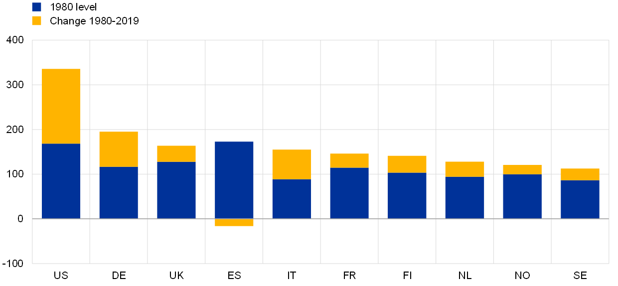
Source: World Inequality Database.
Notes: This chart shows the pre-tax national income of the top 10% of households as a percentage of the pre-tax national income of the bottom 50% of households. Pre-tax national income is defined as the sum of all pre-tax personal income flows accruing to owners of labour and capital, before taking account of the operation of tax/transfer systems, but after taking account of the operation of pension systems.
Income taxation and government transfers have a dampening effect on income inequality, with the precise nature of that impact varying across countries on the basis of their tax systems. If we compare the distribution of disposable income with that of market income for the four largest euro area countries, the United Kingdom and the United States (Chart 2), the dampening effect of direct taxation (e.g. via progressive income taxes) and transfers is evident. The degree of income inequality is indicated by the Gini coefficient, which measures the extent to which the distribution of income among individuals/households deviates from a perfectly equal distribution, with a value of 0 indicating absolute equality and a value of 100 signalling full inequality (whereby the top income group receives all income). Most notably, we can see that the amount of income redistribution carried out by the government is far higher in the European countries (average decline of 20 basis points in the Gini coefficient) than it is in the United States (decline of 14 basis points). However, it is not clear, a priori, to what extent the higher degree of redistribution in Europe can explain the more limited increase in income inequality in the European countries in question (as shown in Chart 1). Two recent studies concluded that the difference between Europe and the United States in terms of the increase in income inequality is driven mainly by market income – i.e. income before redistribution.[5]
Chart 2
Reduction of Gini coefficients through governments’ direct taxes and transfers
(Gini coefficients)
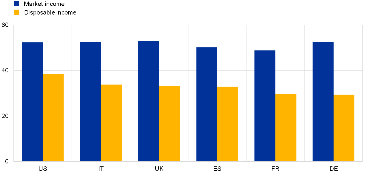
Source: Standardized World Income Inequality Database, versions 8 and 9.[6].
Notes: This chart is based on data for 2017. Market income is broadly defined as income before tax and transfers; disposable income is defined as income after tax and transfers that is available for spending and saving.
Consumption is substantially less concentrated than net wealth, which may suggest that economic well-being is more evenly distributed than wealth. Consumption inequality is sometimes regarded as a better indicator of the standard of living and welfare than income or wealth-based measures.[7] As Chart 3 shows, the Gini coefficient of consumption expenditure is typically lower than that of disposable income, reflecting the fact that higher-income households have a higher saving rate. The recent rise in wealth inequality has been shown to be a result not only of higher (gross) saving rates, but also of higher returns for wealthier households, suggesting that greater concentration of capital income may be an important driver of wealth inequality.[8] The Gini coefficient of net wealth, which is defined as assets (housing, deposits, bonds, equity, etc.) minus liabilities (mortgages, personal loans, etc.), is almost double that of consumption.
Chart 3
Gini coefficients of disposable income, consumption and net wealth
(Gini coefficients)
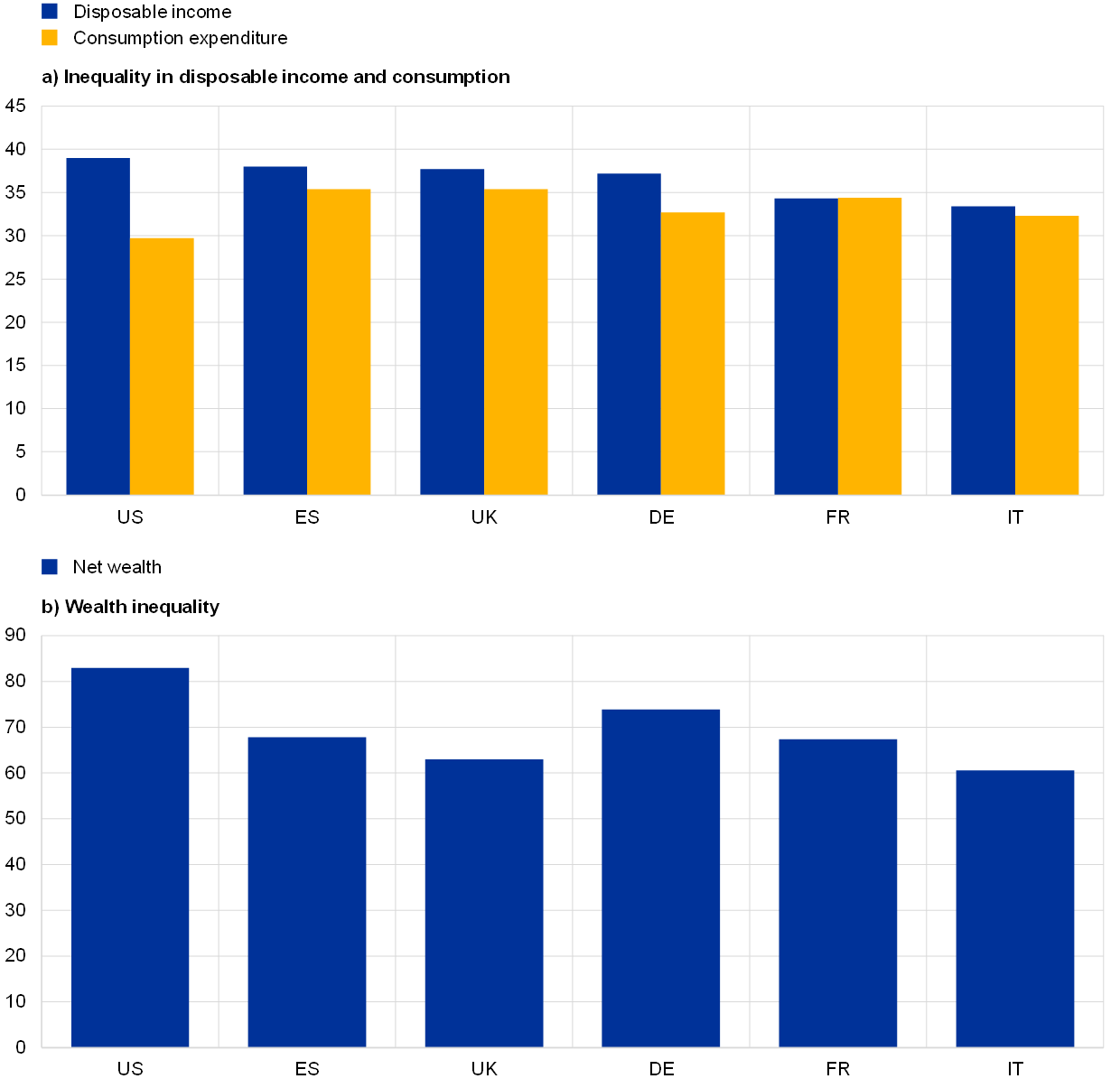
Sources for panel a: Standardized World Income Inequality Database, versions 8 and 9 (net income), for the United States; World Income Inequality Database for consumption in Italy; Eurostat (based on EU Statistics on Income and Living Conditions (EU-SILC)) for all other data.
Sources for panel b: 2020 ECB Household Finance and Consumption Survey (HFCS) for euro area countries; UK Office for National Statistics for the United Kingdom; World Inequality Database (net personal wealth) for the United States.
Note on panel a: Data for European countries relate to the latest available EU-SILC reference year, which is between 2013 and 2018. Note on panel b: All data relate to 2017.
The main factors driving increases in inequality include globalisation, technological progress and changes in taxation. Globalisation and skill-biased technological change have adversely affected the wages and employment of lower‑skilled labour and benefited higher-skilled labour and owners of capital.[9] At the same time, declines in the progressivity of the tax system have contributed to increases in post-tax inequality.[10] A recent study summarised potential drivers of inequality at the various economic stages – i.e. policies in the pre-production stage focusing on people entering the workforce (e.g. as regards access to education or the job market), production policies affecting workers (e.g. as regards unionisation or the minimum wage), and post-production policies redistributing income.[11] Its findings suggest that the rise in income and wealth inequality has been driven mainly by structural policies (e.g. policies on education, taxation and market regulation).
Excessive inequality may entail macroeconomic costs and dampen economic growth. For example, to the extent that it reflects inequality of access to education or finance, economic growth may suffer as a result of the economy failing to use its full potential. Moreover, aggregate demand may be depressed as a result of higher‑income households having a lower propensity to consume.[12] Indeed, empirical studies seem to conclude that very high levels of inequality may well curb economic growth in advanced economies.[13] However, while redistributive policies (e.g. higher tax rates) may limit the degree of inequality, they may also cause distortions that reduce overall welfare. Thus, the socially optimal degree of economic inequality is not easy to determine, reflecting the complex nature of the interaction between its various drivers.
Monetary policy is not likely to be a substantial driver of increases in inequality, but it should not ignore them either. Advanced economies have tended to adopt fairly similar monetary policy strategies in the period since the 1980s, so it seems unlikely that monetary policy is helping to drive the cross-country variation that has been observed. Nevertheless, monetary policy may still need to take those developments into account, especially if they consistently depress aggregate demand or place downward pressure on the natural rate of interest.[14] Governments have instruments at their disposal that are better suited to addressing excessive levels of inequality, such as taxation (e.g. progressive taxes on income, wealth and inheritance), transfers, market regulation, and access to education and health services.
Inequality and the business cycle
The cyclicality of income inequality differs across countries, while wealth inequality tends to be procyclical. While lower-income households tend to be more affected by recessions as a result of the greater sensitivity of their labour income (see below), higher-income households tend to be more exposed to the business cycle as a result of capital income (e.g. profits) making up a larger percentage of their total income. Since the distribution of labour and capital income differs across countries, the cyclicality of income inequality can also differ.[15] Wealth inequality, on the other hand, tends to be mostly procyclical. The procyclicality of profits and equity prices means that equities are not conducive to smooth consumption over the business cycle. With only wealthier households being willing to shoulder such risk (in exchange for a risk premium), that procyclicality helps to explain both the limited levels of participation in the stock market and the substantial equity premium.[16] Consequently, the cyclical properties of certain asset prices can become a longer-term determinant of wealth inequality.
The cyclical sensitivity of earnings differs across households, which gives macroeconomic stabilisation policies a role to play in averting longer-term increases in inequality. Chart 4 reports “worker betas” for the euro area, which measure the elasticity of labour income in relation to changes in aggregate GDP growth.[17] As the chart shows, the labour income of workers in lower-income households is more sensitive to changes in GDP growth (see also Box 1, which focuses specifically on the coronavirus (COVID-19) crisis). For those workers, the welfare costs of business cycles are likely to be substantial, especially as they are less able to smooth consumption as a result of their tighter liquidity and credit constraints. Overall, the cyclical behaviour of earnings suggests that macroeconomic stabilisation policies – whether monetary or fiscal – can play an important role in dampening cyclical increases in income inequality. To the extent that cyclical job losses lead to persistent or even permanent scars on people’s labour market opportunities, these policies can also help to mitigate income and wealth inequality in the longer term.[18]
Chart 4
“Worker betas” across the income distribution in the euro area
(income elasticity of individual workers in relation to GDP growth)
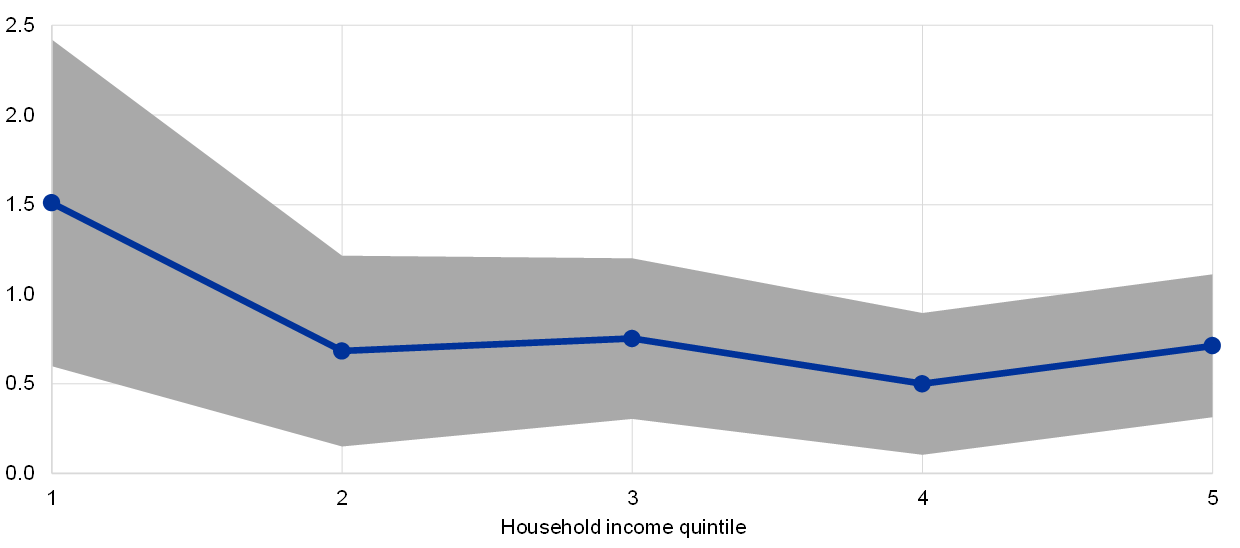
Source: “Household income risk over the business cycle”, Economic Bulletin, Issue 6, ECB, 2019.
Notes: This chart is based on average data for Germany, Spain, France and Italy. It indicates the estimated elasticity of labour income in response to changes in aggregate GDP growth across the household income distribution. Individuals are sorted into income quintiles on the basis of their household income in the two previous years to avoid any spurious correlation between exposure and sorting. Household income is based on EU-SILC variable HY020 (total disposable household income) in the longitudinal data file, with the EU-SILC longitudinal data file clone from the GSOEP being used for Germany. The grey shading indicates 95% confidence intervals.
Box 1
COVID-19 and income inequality in the euro area
While the COVID-19 pandemic has severely reduced the economic well-being of all households, its effects have varied depending on households’ occupations and the structure of their expenditure. This box presents evidence for the euro area on the basis of household-level data on labour income, consumption and saving.
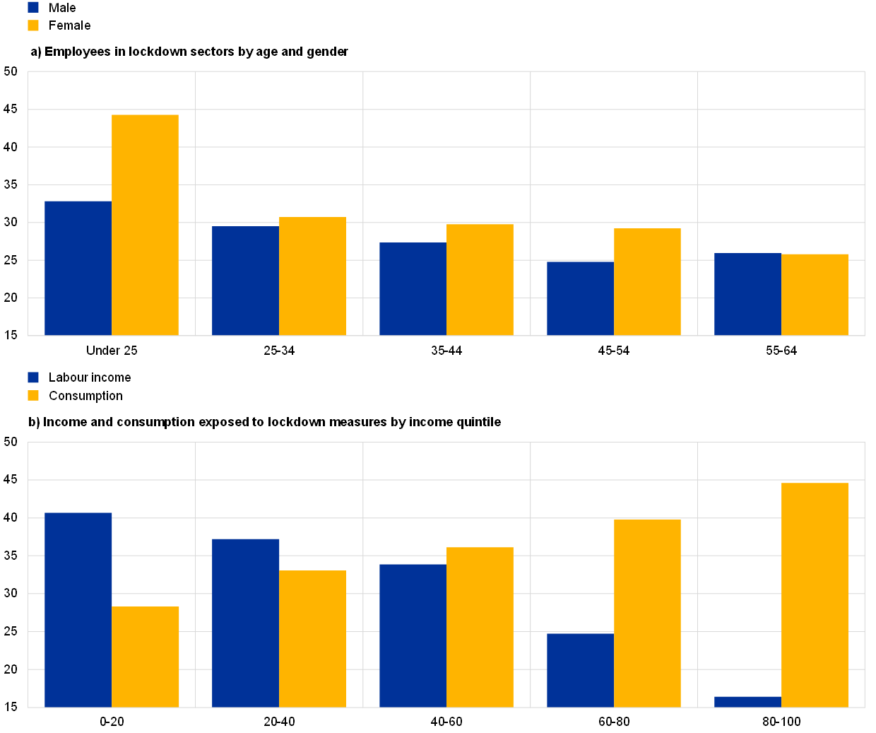
The adverse implications for labour income have been particularly pronounced for younger workers, women and households with lower levels of income. Panel a of Chart A shows, for each age category, the percentage of total employees that work in sectors which have been directly affected by the lockdown restrictions imposed on account of the virus.[19] Those measures have particularly affected sectors where physical distancing rules are difficult to follow, such as hospitality, travel, arts and entertainment. Panel a documents two findings: first, that employees in lockdown-affected sectors are more likely to be younger workers, with the pandemic having an especially strong impact on employees under the age of 25; and second, that women are substantially more likely to work in sectors that have been affected by the lockdown (a finding that holds across nearly all age brackets). Correspondingly, as panel b shows, the effect of COVID-19 is regressive across the income distribution, with the unemployment risk being skewed towards households in lower quintiles. These results are consistent with evidence from other countries indicating that the pandemic is likely to aggravate household inequality. For example, several studies conducted in the United States and the United Kingdom have shown that the percentage of employees working in sectors affected by lockdown measures is particularly high for individuals in the lower part of the income distribution.[20] As a result, the pandemic is likely to amplify existing income inequalities, in line with the findings for previous pandemics.[21]
Chart A
Impact of COVID-19 broken down by age, gender and income quintile
(percentages)
Source for panel a: EU-SILC (2017 data for Ireland and Slovakia; 2018 data for all other countries).
Sources for panel b: EU-SILC (2017 data for Ireland and Slovakia; 2018 data for all other countries) and Eurostat Household Budget Survey.
Notes on panel a: This panel shows, for each age category, the percentage of total employees (broken down by gender) that are working in lockdown sectors. The following sectors are considered to be subject to lockdown measures: wholesale and retail trade, and repair of motor vehicles and motorcycles; transport and storage; accommodation and food service activities; and arts, entertainment and recreation (sectors G, H, I and R respectively in the Statistical Classification of Economic Activities in the European Community (NACE classification)).
Notes on panel b: This panel shows, for each income quintile, the percentage of total income and consumption that is exposed to lockdown measures. Exposed consumption includes spending on restaurant food, transport services, holidays, hotels and cultural services, as well as postponable spending (such as purchases of motor vehicles, clothing, footwear, furnishings and furniture).
In contrast to labour income, the decline in household consumption has been particularly pronounced in the upper parts of the income distribution, with high-income households strongly reducing their spending on non-essentials, which make up almost 45% of the total expenditure of households in the top quintile.[22] Those households have made a disproportionate contribution to the substantial increase seen in the aggregate saving rate, both because goods and services affected by lockdown measures make up a larger percentage of their total consumption, and because their income has been less affected.
Fiscal policies, combined with the ECB’s monetary policy measures, have helped to mitigate the economic fallout from the COVID-19 crisis. While the ECB’s accommodative monetary policy has ensured favourable financing conditions for the whole economy, targeted fiscal transfers (e.g. job retention schemes) have softened the blow for those households that have been most affected.
3 Monetary policy and household inequality
How does monetary policy affect income and wealth inequality?
The economic literature has identified three main channels through which a change in the monetary policy stance can have distributional consequences for household wealth and income. The first is the savings remuneration (and cost of debt) channel, which stems from differences in the size and composition of household balance sheets. Because of those differences, a change in interest rates will have opposing effects on the economic conditions of net borrowers and net savers. The second is the asset price channel, which stems from the heterogeneity of household portfolios and the diverse capital gains (or losses) that are produced when the monetary policy stance changes. In this respect, asset price movements induced by expansionary policies are more likely to benefit the wealthy (and, in some cases, the middle class) to the extent that they hold longer-term assets (as explained in more detail in Box 3). The third channel relates to household income and arises because the elasticity of employment relative to the business cycle is heterogeneous across individuals and dependent on individual characteristics.
Monetary policy and inequality: empirical evidence from the euro area
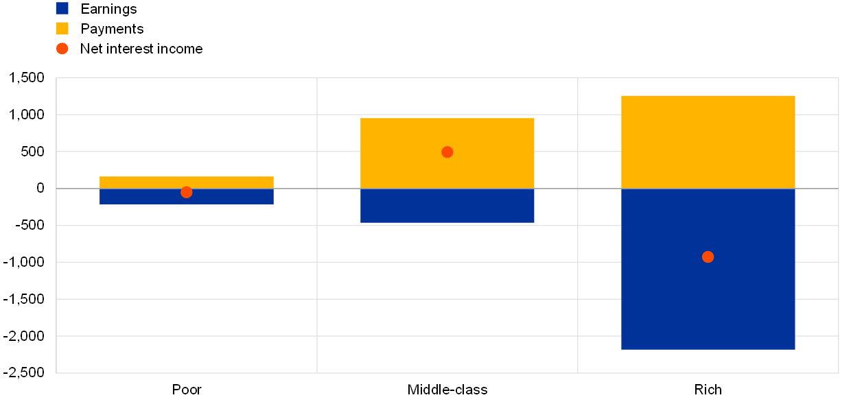
Net interest income reacts differently across households in response to a reduction in the interest rate. This mainly depends on the extent to which households’ interest-bearing assets have short maturities and their mortgages have adjustable rates.[23] As the estimates in Chart 5 show, the net interest income of poorer households has not been greatly affected by the fall in interest rates, since they tend to have low levels of both debt and interest-bearing assets. In contrast, the net interest income of middle-class households has increased as interest rates have declined, mainly because they have relatively high levels of mortgage debt. Finally, richer households have recorded a net loss of interest income, since they tend, on average, to be less indebted.[24] Thus, the direct impact of lower interest rates does not seem to increase income inequality.
Chart 5
Changes in net interest income across the income and wealth distribution
(EUR per household; change in annual net interest income, 2007-19)
Source: Dossche et al., op. cit.
Notes: “Rich” households are defined as the top 20% of the net wealth distribution (financial and non-financial wealth); “middle-class” households are the 60% of the overall population that are at the top of the income distribution of non-rich households; “poor” households are the 20% of the overall population that are at the bottom of the income distribution of non-rich households.
An easing of monetary policy affects household labour income via two main channels. The first involves unemployed people finding jobs – and generally experiencing a substantial increase in income as a result (the earnings heterogeneity channel).[25] The probability of this outcome depends on people’s demographic characteristics (age, level of education, marital status, number of children, etc.). The second involves increases in the wages of employed individuals (the income composition channel).
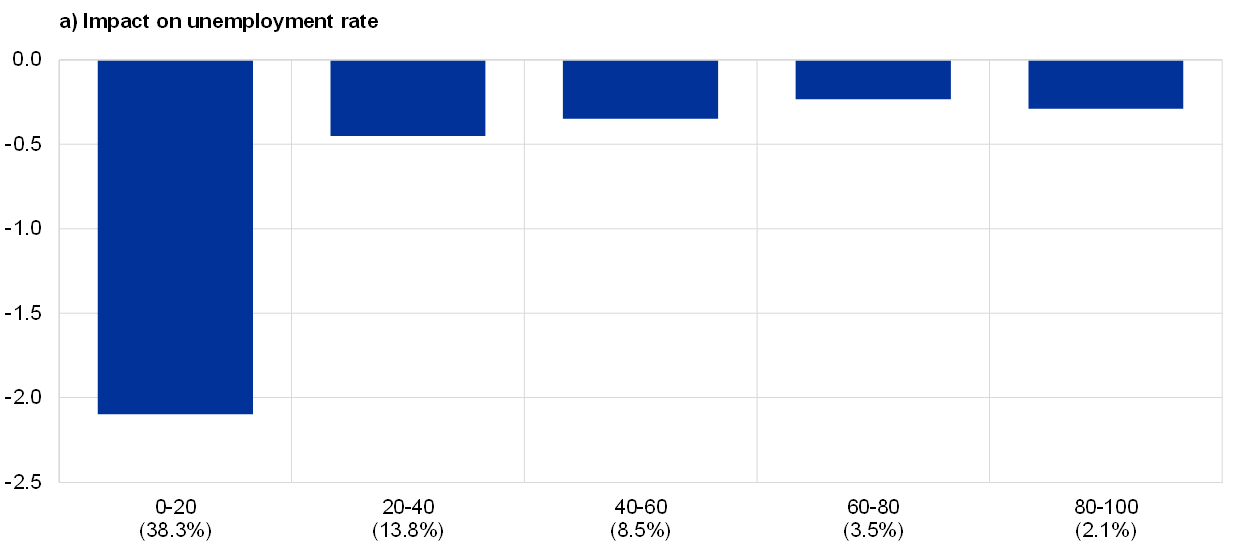
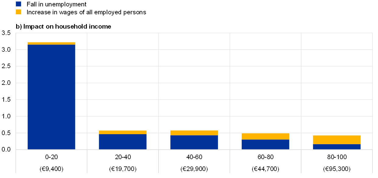
The easing of monetary policy through the ECB’s asset purchase programme (APP) has substantially reduced the unemployment rate in the lower part of the income distribution.[26] Panel a of Chart 6 estimates the decline in the unemployment rate which can be attributed to the APP for each of the five quintiles of the income distribution, calculating those declines four quarters after the APP shock (which is represented here by an unanticipated drop in the interest rate term spread – the difference between long and short-term interest rates – of 30 basis points). The aggregate decline in the unemployment rate (which totals around 0.7 percentage points) affects individuals very differently, mainly benefiting households with incomes in the lowest quintile. Their unemployment rate falls by more than 2 percentage points, while the unemployment rates of all other income quintiles fall by less than 0.5 percentage points.
Chart 6
Impact of monetary easing via the APP
(percentage points)
(percentages)
Source: Lenza, M. and Slačálek, J., op. cit.
Notes: Panel a shows the decline in the unemployment rate for the various quintiles of the household income distribution four quarters after the materialisation of the APP shock. The figures in parentheses in that panel show the initial unemployment rate for each quintile. Panel b shows the percentage change in mean income for the various quintiles, as well as breaking that change down into the extensive margin (earnings heterogeneity channel) and the intensive margin (increase in wages). The figures in parentheses in that panel show the initial level of mean gross household income for each quintile. For the purposes of this chart, the euro area has been modelled by aggregating data for Germany, Spain, France and Italy.
The decline in unemployment is found to be a substantial driver of wage increases across the income distribution, particularly in the lower quintiles. Panel b of Chart 6 breaks the overall increase in mean income down into (i) the part that is due to the decline in unemployment (the earnings heterogeneity channel) and (ii) the part that is due to the increase in wages for all workers (the income composition channel). The earnings heterogeneity channel has a particularly strong impact in the bottom quintile, where wage growth plays a very small role. However, it also accounts for the bulk of the total impact on income in three of the other four quintiles (with the top quintile being the exception).
Overall, the labour market impact of the APP is estimated to result in some reduction in income inequality. Changes in unemployment rates substantially affect household incomes, with incomes increasing considerably on account of households either starting to or continuing to earn wages (instead of receiving unemployment benefits). The mean income of the lowest quintile rises by more than 3%, while those of other quintiles increase by around 0.5%.
The APP also has an impact on the distribution of wealth via the portfolio composition channel. The APP boosts the value of some household assets (stocks, bonds and housing), which affects around two-thirds of all households who hold them. Because stocks are mostly held by wealthier households, an increase in stock prices tends, by itself, to lead to an increase in wealth inequality. However, that increase is offset by the parallel rise in house prices. Housing is fairly evenly distributed across euro area households, with a large percentage (around 60%) owning their main residence.[27] Moreover, housing accounts for around 70-80% of the total value of all household assets.[28] When the effects on stock prices and house prices are combined, the Gini coefficient of net wealth – a broad measure of inequality – remains broadly unchanged.
These findings are consistent with the growing body of literature estimating the distributional effects of monetary policy.[29] Two recent studies, for example, concluded that the overall effect that unconventional monetary policy measures have had on income and wealth inequality has been fairly small.[30] The Deutsche Bundesbank, meanwhile, has concluded that non-standard monetary policy measures have probably reduced income inequality, while their impact on the distribution of wealth is less clear.[31] For the Portuguese economy, the Banco de Portugal has found that while increases in house prices tend to reduce wealth inequality, rises in the value of self-employment businesses and marketable financial wealth increase it.[32] Meanwhile, recent work focusing on cross-racial differentials in the United States has found that while an accommodative monetary policy stance tends to reduce cross-racial differences in unemployment (and thus earnings), it exacerbates wealth differentials.[33]
Box 2
Monetary policy and regional inequality
In many parts of the world, the economic fortunes of poorer and richer regions have diverged in recent years. In Europe, for example, regional disparities have intensified since the start of EMU, notably on account of hysteresis following the global financial crisis.[34] A recent paper confirms that divergent dynamics emerged in the euro area after the financial crisis, in that the upper parts of the income distribution experienced a solid recovery following the contraction in 2009, whereas the lower parts experienced continued declines in GDP per capita.[35] Moreover, a recent box in the Economic Bulletin documents the same type of divergence in labour markets.[36]
That increase in regional inequality has attracted attention, but the contribution made by monetary policy has not yet been considered. Most of the debate has focused on tax and transfer systems or underlying shifts in economic structures as the key forces shaping the dynamics of regional inequality.[37] However, it is natural to wonder whether those forces have been exacerbated or mitigated by economic policies at the macro level. And of the various policy domains, monetary policy is an interesting candidate, given its important role in steering macroeconomic outcomes over the last decade.
In that context, this box seeks to shed light on the dynamic impact that exogenous changes in short-term policy rates have had on the GDP of cities and other regional units in the euro area. In deriving those exogenous changes, the empirical model that is used here controls for key macroeconomic variables (such as euro area GDP and HICP inflation) that typically form part of the central bank reaction function. Thus, the identification strategy posits that, controlling for macro conditions, monetary policy does not respond to economic activity at the regional level.
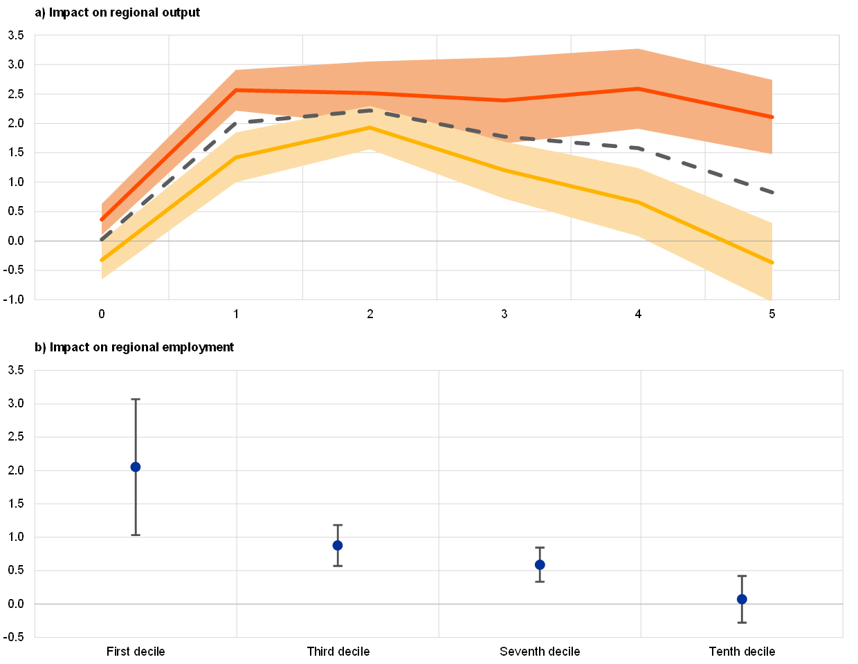
The results point to pronounced heterogeneity in the regional patterns of monetary policy transmission. For instance, panel a of Chart A compares the dynamic response of regional output to a monetary policy shock at the 5th and 95th percentiles of the distribution. In both parts of the distribution, output expands following the rate cut, but the expansion is much stronger at the lower end. Moreover, that gap widens over time. Indeed, while output in the upper part of the distribution returns to its previous level, the impact on output proves to be persistent in the lower part. As a consequence, the easing of monetary policy mitigates regional inequality and policy tightening aggravates it.
Chart A
Impact of monetary policy at regional level
(percentages)
Source: Hauptmeier et al., op. cit.
Notes on panel a: This panel shows the impact that a 100 basis point interest rate cut has on regional GDP (in percentages). The horizontal axis indicates the IRF horizon (in years). Lines denote point estimates, and shaded areas denote 90% confidence intervals. The red line depicts estimates for the 95th percentile of the conditional distribution of GDP at regional level; the yellow line depicts the 5th percentile; the dashed line depicts the mean.
Notes on panel b: This panel shows the impact that a 100 basis point interest rate cut has on employment five years later (in percentages) across various deciles of the distribution of regional per capita GDP. Dots indicate point estimates; bars denote 90% confidence intervals. Regions are defined in accordance with Eurostat’s NUTS 3 classification.
These findings illustrate the role that is played by the distributional effects of monetary policy (including along geographical lines). Moreover, while discussions regarding the unequal geographical impact of euro area monetary policy typically focus on cross-country differences, this analysis shows that the issue of geographical heterogeneity runs deeper than that: interregional heterogeneity becomes more accentuated at more granular geographical levels, and that heterogeneity, in turn, profoundly alters the implications of a given monetary policy stance in different parts of the economy.
In line with a long-standing body of literature,[38] Hauptmeier et al. (op. cit.) point to labour markets as a likely driver of such developments: employment’s response to monetary policy shocks is particularly persistent, and long-lasting effects are particularly pervasive across the distribution of regional per capita GDP. As panel b of Chart A shows, statistically significant and economically relevant employment effects can still be seen five years after a monetary policy shock, right up to the seventh decile of the distribution of regional per capita GDP. Overall, these findings add to a growing body of literature suggesting that monetary policy may trigger long-lasting effects, with greater implications for welfare than if it merely smoothed out temporary fluctuations in economic activity.[39]
4 Heterogeneity and the transmission of monetary policy to household spending
Whereas the previous section focused on the impact that monetary policy has on income and wealth inequality, this section looks at the ways in which the distribution of income and wealth shapes the transmission of monetary policy to households. Specifically, it estimates the manner in which the transmission of monetary policy to consumption varies across individual households on the basis of the structure of their income and wealth, their marginal propensity to consume (MPC) and the ways in which their income responds to aggregate shocks.
Direct and indirect transmission channels for monetary policy
The effects that monetary policy has on individual households can be grouped together in two broad categories: direct and indirect.
Direct effects are the immediate, partial-equilibrium consequences of the change in interest rates. These include the impact that the different interest rate paths have on households’ net financial income (net interest rate exposure). This is often the main channel highlighted by commentators. It is heterogeneous across households, depending on the composition of their asset and liability portfolios. For example, a reduction in policy rates will reduce interest payments for households with outstanding debt (as explained above), especially if their loans have variable rates. It will also reduce the financial income of households that are not indebted, but hold short-maturity assets (whose real returns will temporarily fall). A second direct effect of monetary policy involves changes to households’ saving incentives (intertemporal substitution). This effect is also heterogeneous, since it mostly applies to households that have a stock of liquid savings and are therefore able to temporarily adjust them without paying large transaction costs.
Indirect effects operate through the general equilibrium responses of prices and wages (and thus labour income and employment). When policy rates are reduced, the resulting direct increase in household expenditure (and investment by firms) leads to an increase in output and exerts upward pressure on employment and wages. This indirect effect, which works via the increase in labour income (especially in the lowest quintile, as described in the previous section), leads to additional increases in aggregate demand. It, too, will have heterogeneous consequences to the extent that different sources of earnings (e.g. wages versus income from private businesses) or different pools of unemployed workers (e.g. low versus high‑skilled individuals) display differing degrees of elasticity in their response to the change in aggregate expenditure.
Empirical estimates for the euro area
The economic literature is increasingly finding evidence that individual households behave differently in terms of the ways in which their consumption responds to income shocks – i.e. that households differ in their marginal propensity to consume.[40] Authors have found it useful to classify households on the basis of the amount of liquid assets that they hold. Households with few liquid assets tend to have large MPCs, and they are often described as “hand-to-mouth”, because they tend to consume all of their income.[41] They can be either “poor” (if they do not own any assets) or “wealthy” (if they have positive illiquid wealth (e.g. they own their home), but have very limited liquid assets and large spending commitments (e.g. a sizable mortgage)).[42] In contrast, unconstrained (or “non-hand-to-mouth”) households behave in line with the permanent income hypothesis: their spending patterns remain essentially unchanged in response to a transitory increase in income. On the basis of that classification, 10% of euro area households are “poor hand-to-mouth”, 12% are “wealthy hand-to-mouth” and 78% are “non-hand-to-mouth”.
In order to estimate the size of the various transmission channels to consumption, we need both aggregate and micro-level data on household portfolios and income.[43] As regards aggregate data, vector autoregressive models can be used to estimate the manner in which aggregate earnings and asset prices respond to monetary policy. In addition, micro-level data are necessary in order to quantify households’ exposure to interest rate risk, inflation risk, asset prices and labour income risk.
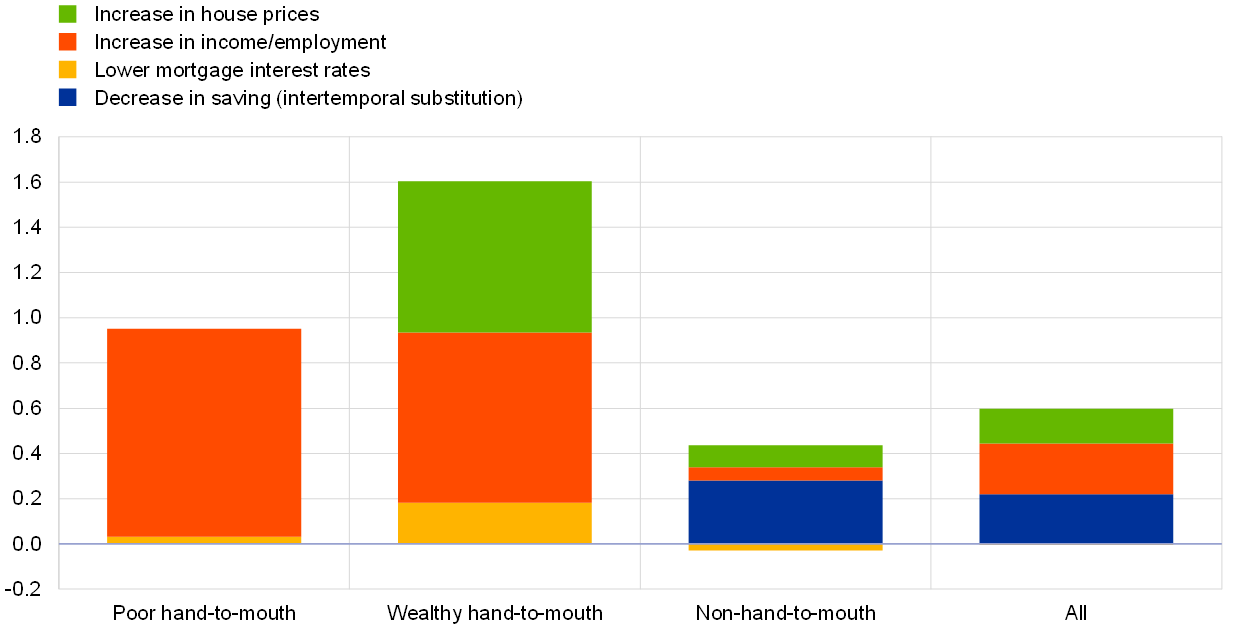
As Chart 7 shows, spending by hand-to-mouth households increases more strongly than spending by non-hand-to-mouth households in response to an easing of monetary policy. A 100 basis point cut in real interest rates increases consumption by poor hand-to-mouth households by almost 1% and increases consumption by wealthy hand-to-mouth households by 1.6%, while consumption by other households increases by just 0.5%.
Chart 7
Estimated impact on consumption of a 100 basis point cut in real interest rates in the euro area
(percentages)
Source: Slačálek et al., op. cit.
Notes: This chart shows the impact that a 100 basis point cut in real interest rates has on consumption one year later, breaking that impact down into (i) the standard intertemporal substitution effect (which reduces saving), (ii) the cash flow channel resulting from the decline in mortgage interest rates, (iii) the income channel resulting from increases in employment and wages, and (iv) the housing wealth effect caused by increases in house prices. The size of those effects varies depending on households’ wealth. In the euro area, 10% of households are poor hand-to-mouth, 12% are wealthy hand-to-mouth and 78% are non-hand-to-mouth. For the purposes of this chart, the euro area has been modelled by aggregating data for Germany, Spain, France and Italy.
When monetary policy is eased, consumption by hand-to-mouth households is mostly stimulated via indirect effects, while consumption by non‑hand‑to‑mouth households is mostly stimulated via the intertemporal substitution channel. The impact of indirect effects is heavily skewed towards hand-to-mouth households, as they tend to have lower incomes and benefit disproportionately from the new jobs and the corresponding employment income. The effect that this channel has on consumption is amplified because those households have larger MPCs than other households. The intertemporal substitution channel plays a major role for non-hand-to-mouth households that have significant stocks of savings, while the other transmission channels (operating through changes in house prices and, in particular, changes in net financial income) play a smaller role in quantitative terms.[44]
Accounting for differences across households is important when assessing the impact that monetary policy has on aggregate consumption. In general, monetary policy has only a temporary impact on the economy, with its effects tending to dissipate in the long run. Thus, other factors, such as globalisation or the ways in which individual tax systems redistribute income and wealth (e.g. by means of progressive taxation), will tend, in the long run, to be more important drivers of inequality than monetary policy. However, our results indicate that monetary policy can indeed be effective in supporting household consumption during downturns.
Box 3
Capital gains, welfare and consumption
The recent lowering of interest rates by means of the reduction of policy rates and net asset purchases has contributed to capital gains for longer-term assets.[45] This raises two questions. First, to what extent have those capital gains contributed to wealth inequality? And second, to what extent have they generated wealth effects on consumption, thereby stimulating aggregate activity? Economic theory suggests that finding answers to these questions may not be particularly straightforward.
It is not true, for example, that equity holders always benefit via capital gains when interest rates fall.[46] Indeed, one needs to look at whether their assets have longer durations than their liabilities. Unhedged interest rate exposures (UREs) – the difference between all maturing assets and liabilities at a given point in time – are the best measure of households’ balance sheet exposure to interest rate changes. People whose financial wealth is invested primarily in short-term deposits tend to have positive UREs, while those with large variable rate mortgage liabilities tend to have negative UREs. A fall in interest rates redistributes wealth away from the first group towards the second.
Importantly, liabilities also include consumption plans, and assets also include human capital. Thus, capital gains resulting from lower interest rates have no effect on households whose dividend streams are equal to their planned consumption. Instead, lower interest rates benefit households who hold long-term assets for the purpose of financing short-term consumption (e.g. older households who hold equity shares or long-term bonds), through the capital gains that they generate. And they hurt households who finance a long-term consumption stream (e.g. retirement) using short-term assets (e.g. pre-retirement income), by lowering the rate at which they can invest their earnings. These conclusions have been derived from a stylised model, and some of the underlying assumptions may not, in practice, always apply (e.g. owing to bequest motives). Overall, however, economic theory makes it clear that even if two different households hold the same amount of wealth and their wealth is composed in exactly the same way, the welfare effects of capital gains on their portfolios may vary, depending on their consumption and investment plans.
Likewise, rising house prices on account of a fall in interest rates should generate a heterogeneous wealth effect on consumer spending. One should expect to see older home-owning households increasing their consumption when house prices rise.[47] Again, however, households will alter their consumption in different ways, depending on their investment plans. A recent study provides empirical confirmation of those intuitive conclusions.[48] Using survey data from the Netherlands, it finds significant heterogeneity in wealth effects, with more than 90% of homeowners reporting no reaction to either positive or negative housing wealth shocks. This corresponds to an average wealth effect of between 2% and 5%, in line with econometric estimates linking changes in aggregate housing wealth with aggregate realised consumption.[49] Moreover, it also finds, in line with economic theory, that the wealth effects of rising house prices are larger for older households (panel a of Chart A). Finally, it finds that the increase in consumption which stems from a positive housing wealth shock is greater (in absolute terms) than the decline in consumption which is triggered by a negative shock of an equal size (panel b of Chart A). This is consistent with the existence of a collateral channel mechanism over and above the pure wealth effect. Increases in the value of people’s homes allow additional borrowing and spending, while declines in value do not necessarily require households to reduce their borrowing, given that the loan-to-value constraint is only binding at the time of the loan’s origination.
Chart A
The relationship between wealth effects and age
(percentages)
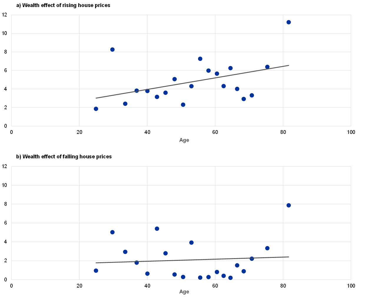
Source: Christelis et al., op. cit. in footnote 48.
Overall, recent literature suggests that capital gains and greater wealth inequality on account of declines in interest rates do not automatically translate into increases in the welfare or consumption of benefiting households. In order to acquire a thorough understanding of the interaction between monetary policy and inequality, more research needs to be carried out into the role played by households’ investment plans in this regard.[50]
5 Conclusion
In many advanced economies, inequality has been on the rise for several decades, mainly as a result of factors other than monetary policy. While income and wealth inequality have tended to rise in most advanced economies, there is significant cross-country heterogeneity, both in the extent to which inequality has increased and in the current levels of inequality. In the euro area, for example, income and wealth inequality are both generally lower than in the United States. While some drivers of rising inequality are common to most countries (e.g. globalisation), policies other than monetary policy have been key in explaining those cross-country differences. After all, most advanced economies have, since the 1980s, tended to adopt fairly similar monetary policy frameworks, with inflation remaining low and stable. What is more, to the extent that cyclical job losses lead to permanent scars on people’s employability, monetary policy has actually helped to prevent longer-term increases in income and wealth inequality on account of the business cycle.
Indeed, the easing of monetary policy would seem, overall, to have dampened economic inequality in recent years. The direct effects of such easing are heterogeneous as a result of differences in households’ ownership of housing and, accordingly, the prevalence of mortgages. More importantly, the easing of monetary policy clearly has an inequality-reducing impact via its indirect effects, resulting in increased employment for lower-income households in particular. While the ECB has neither the mandate nor the instruments that it would need to specifically target the distribution of income and wealth, its current policies generally seem to have an equalising impact through their contribution to macroeconomic stabilisation.
The heterogeneity of households plays a key role in the transmission of monetary policy. As households differ substantially in terms of the composition of their wealth, the sensitivity of their income to the business cycle, and their propensity to consume, the distribution of income and wealth plays a key role in shaping the transmission of monetary policy to economic activity and inflation. While recent improvements to models and data have contributed to a better understanding of this part of the monetary transmission channel, several puzzles remain (as Box 3 showed). Consequently, the ECB continues, like many other central banks, to invest in new macroeconomic models and data sources in order to improve its understanding of the ways in which its policies affect inequality and the manner in which household heterogeneity shapes the transmission of its policies.
- See Piketty, T., Capital in the Twenty-First Century, Harvard University Press, 2013. Differences in income and wealth are typically correlated with various economic characteristics (such as people’s level of education, professional experience and skills). However, those economic characteristics are not the only drivers of economic inequality. People’s income and wealth are also correlated with various sociological characteristics (such as their age, gender, race, marital status and religion). In addition, public policies (e.g. as regards tax, education, housing and urbanisation) and social norms (e.g. discrimination) interact with those economic and sociological characteristics. Thus, the drivers of inequality are manifold and lie at the intersection of economics, sociology and public policy.
- Inequality was, for example, one of the topics that came up most at listening events organised in the context of the review of the ECB’s monetary policy strategy, with many participants arguing that monetary policy should play a more prominent role in addressing inequality. See the ECB’s summary report on that listening exercise: https://www.ecb.europa.eu/home/search/review/html/ecb.strategyreview001.en.html
- See Yellen, J., “Macroeconomic Research After the Crisis”, speech delivered at the Federal Reserve Bank of Boston, 14 October 2016.
- See, for example, Ahn, S., Kaplan, G., Moll, B., Winberry, T. and Wolf, C., “When Inequality Matters for Macro and Macro Matters for Inequality”, NBER Macroeconomics Annual, Vol. 32, 2017, pp. 1-75.
- See Blanchet, T., Chancel, L. and Gethin, A., “Why is Europe more equal than the United States?”, WID Working Papers, No 2020/19, 2020; and Bozio, A., Garbinti, B., Goupille-Lebret, J., Guillot, M. and Piketty, T., “Predistribution vs. Redistribution: Evidence from France and the U.S.”, CEPR Discussion Papers, No 15415, 2020.
- See Solt, F., “The Standardized World Income Inequality Database, Versions 8-9”, 2019.
- See Attanasio, O. and Pistaferri, L., “Consumption Inequality”, Journal of Economic Perspectives, Vol. 30(2), 2016, pp. 3-28. The authors of that article also warn against focusing on total consumption, on the basis that consumption baskets tend to differ greatly across socio-economic groups.
- See Fagereng, A., Guiso, L., Malacrino, D. and Pistaferri, L., “Heterogeneity and persistence in returns to wealth”, Econometrica, Vol. 88, 2020, pp. 115-170; and Fagereng, A., Holm, M.B., Moll, B. and Natvik, G., “Saving Behavior Across the Wealth Distribution: The Importance of Capital Gains”, NBER Working Papers, No 26588, 2019.
- See Bourguignon, F., “World changes in inequality: an overview of facts, causes, consequences and policies”, BIS Working Papers, No 654, 2017; and Rodrik, D., Has Globalization Gone Too Far?, Institute for International Economics, 1997.
- See Chancel, L., “Ten facts about inequality in advanced economies”, WID Working Papers, No 2019/15, 2019.
- See Blanchard, O. and Rodrik, D. (eds.), Combating Inequality: Rethinking Government's Role, MIT Press, 2021.
- See, for example, Mian, A., Straub, L. and Sufi, A., “Indebted Demand”, mimeo, Harvard University, 2019, which looks at the marginal propensity to consume out of permanent income.
- See, for instance, the overview in Ostry, J., Berg, A. and Tsangarides, C., “Redistribution, Inequality, and Growth”, IMF Staff Discussion Notes, No SDN/14/02, 2014.
- See Rachel, L. and Summers, L., “On Secular Stagnation in the Industrialized World”, Brookings Papers on Economic Activity, spring 2019, pp. 1-54.
- See Clemens, M., Eydam, U. and Heinemann, M., “Inequality over the Business Cycle – The Role of Distributive Shocks”, DIW Discussion Papers, No 1852, 2020.
- See Guvenen, F., “A Parsimonious Macroeconomic Model for Asset Pricing”, Econometrica, Vol. 77, 2009, pp. 1711-1750.
- See Castañeda, A., Dı́az-Giménez, J. and Rı́os-Rull, J.-V., “Exploring the income distribution business cycle dynamics”, Journal of Monetary Economics, Vol. 42, 1998, pp. 93-130; and Guvenen, F., Schulhofer-Wohl, S., Song, J. and Yogo, M., “Worker Betas: Five Facts about Systematic Earnings Risk”, American Economic Review, Vol. 107(5), 2017, pp. 398-403. See also the box entitled “Household income risk over the business cycle”, Economic Bulletin, Issue 6, ECB, 2019. While this pattern may be somewhat less pronounced at the level of the euro area as a whole, that box documents significant variation across larger euro area countries, which may potentially be related to differences in labour market institutions.
- . See Heathcote, J., Perri, F. and Violante, G., “The Rise of US Earnings Inequality: Does the Cycle Drive the Trend?”, Review of Economic Dynamics, Vol. 37, Supplement 1, 2020, pp. S181-S204.
- The following sectors are classified as being subject to lockdown measures: wholesale and retail trade, and the repair of motor vehicles and motorcycles; transport and storage; accommodation and food service activities; and arts, entertainment and recreation (in line with Joyce, R. and Xu, X., “Sector shutdowns during the coronavirus crisis: which workers are most exposed?”, Briefing Note BN278, Institute for Fiscal Studies, 2020).
- See Béland, L.-P., Brodeur, A. and Wright, T., “COVID-19, Stay-At-Home Orders and Employment: Evidence from CPS Data”, IZA Discussion Papers, No 13282, May 2020; Mongey, S., Pilossoph, L. and Weinberg, A., “Which workers bear the burden of social distancing policies?”, Covid Economics, Issue 12, 2020, pp. 69-86; and Joyce, R. and Xu, X., op. cit.
- See Furceri, D., Loungani, P., Ostry, J. and Pizzuto, P., “Will Covid-19 affect inequality? Evidence from past pandemics”, Covid Economics, Issue 12, 2020, pp. 138-157.
- “Non-essentials” are defined here as items that are subject to lockdown measures, which include spending on restaurant food, transport services, holidays, hotels and cultural services, as well as postponable spending (such as purchases of motor vehicles, clothing, footwear, furnishings and furniture).
- See Auclert, A., “Monetary Policy and the Redistribution Channel”, American Economic Review, Vol. 109(6), 2019, pp. 2333-2367; and Tzamourani, P., “The Interest Rate Exposure of Euro Area Households”, European Economic Review, forthcoming.
- See Dossche, M., Hartwig, J. and Pierluigi, B., “The redistribution of interest income in the euro area, 2007-2019”, mimeo, 2020.
- Similarly, workers who avoid being made redundant do not experience a loss of income (which they would otherwise do).
- See Lenza, M. and Slačálek, J., “How does monetary policy affect income and wealth inequality? Evidence from quantitative easing in the euro area”, Working Paper Series, No 2190, ECB, October 2018. For more information on the APP, see: https://www.ecb.europa.eu/mopo/implement/app/html/index.en.html
- See Adam, K. and Tzamourani, P., “Distributional consequences of asset price inflation in the Euro Area”, European Economic Review, Vol. 89, 2016, pp. 172-192.
- The impact on households also varies depending on the structure and size of their assets and liabilities: while highly leveraged households (who often have low levels of net wealth) benefit more than wealthy households, households with few assets gain very little (or nothing at all).
- See, for example, Colciago, A., Samarina, A. and De Haan, J., “Central Bank Policies and Income and Wealth Inequality: A Survey”, Journal of Economic Surveys, Vol. 33, 2019, pp. 1199-1231.
- See Casiraghi, M., Gaiotti, E., Rodano, L. and Secchi, A., “A ‘reverse Robin Hood’? The distributional implications of non-standard monetary policy for Italian households”, Journal of International Money and Finance, Vol. 85, 2018, pp. 215-235; and Bunn, P., Pugh, A. and Yeates, C., “The Distributional Impact of Monetary Policy Easing in the UK Between 2008 and 2014”, Staff Working Papers, No 720, Bank of England, 2018. The first of those two papers, which uses Italian data, also finds that non‑standard measures do not hurt savers, as the decline in the remuneration of assets is offset by support for labour income and capital gains.
- See Deutsche Bundesbank, “Distributional Effects of Monetary Policy”, Monthly Report, September 2016, pp. 13-36.
- See Banco de Portugal, “Distribution Mechanisms of Monetary Policy in the Portuguese Economy”, Economic Bulletin, May 2017, pp. 93-110.
- See Bartscher, A., Kuhn, M., Schularick, M. and Wachtel, P., “Monetary Policy and Racial Inequality”, CEPR Discussion Papers, No 15734, January 2021. The main reason for the adverse effect on wealth differentials is that black households in the United States are less likely to hold equity and own a house than white households.
- See Hudecz, G., Moshammer, E. and Wieser, T., “Regional disparities in Europe: should we be concerned?”, ESM Discussion Papers, No 13, July 2020.
- See Hauptmeier, S., Holm-Hadulla, F. and Nikalexi, K., “Monetary policy and regional inequality”, Working Paper Series, No 2385, ECB, March 2020.
- See the box entitled “Regional labour market developments during the great financial crisis and subsequent recovery”, Economic Bulletin, Issue 4, ECB, 2020.
- See Austin, B., Glaeser, E. and Summers, L., “Saving the Heartland: Place-Based Policies in 21st Century America”, Brookings Papers on Economic Activity, spring 2018.
- See, for instance, Blanchard, O. and Summers, L., “Hysteresis and the European Unemployment Problem”, NBER Macroeconomics Annual, Vol. 1, 1986, pp. 15-78.
- See, for example, Blanchard, O., “Should we reject the natural rate hypothesis?”, Journal of Economic Perspectives, Vol. 32(1), 2018, pp. 97-120; and Jordà, Ò, Singh, S.R. and Taylor, A.M., “The Long-Run Effects of Monetary Policy”, NBER Working Papers, No 26666, 2020.
- Studies have tended to approach this issue in one of two ways. The first involves examining real life events (such as unexpected tax rebates for households), measuring the consumption response to income shocks using survey data (see, for example, Jappelli, T. and Pistaferri, L., “The Consumption Response to Income Changes”, Annual Review of Economics, Vol. 2, 2010, pp. 479‑506). The second involves surveys, whereby individuals are asked how their spending would respond in hypothetical or actual scenarios (see, for example, Jappelli, T. and Pistaferri, L., “Fiscal Policy and MPC Heterogeneity”, American Economic Journal: Macroeconomics, Vol. 6(4), 2014, pp. 107-136; and Christelis, D., Georgarakos, D., Jappelli, T., Pistaferri, L. and Van Rooij, M., “Asymmetric Consumption Effects of Transitory Income Shocks”, The Economic Journal, Vol. 129, Issue 622, 2019, pp. 2322‑2341).
- Essentially, hand-to-mouth households hold either (i) positive net liquid assets that are worth less than two weeks of income or (ii) negative net liquid assets that are worth less than two weeks of income minus their credit limit.
- See, for example, Kaplan, G., Moll, B. and Violante, G., “Monetary Policy According to HANK”, American Economic Review, Vol. 108(3), 2018, pp. 697-743; and Weidner, J., Kaplan, G. and Violante, G., “The Wealthy Hand-to-Mouth”, Brookings Papers on Economic Activity, Vol. 48, spring 2014, pp. 77‑153.
- This section summarises the main results of Slačálek, J., Tristani, O. and Violante, G., “Household Balance Sheet Channels of Monetary Policy: A Back of the Envelope Calculation for the Euro Area”, Journal of Economic Dynamics & Control, Vol. 115, 2020, Article 103879.
- House prices affect consumption primarily via the easing of collateral constraints, allowing households to borrow more in order to finance consumption. The impact of this effect is skewed towards constrained households (see, for example, Paiella, M. and Pistaferri, L., “Decomposing the Wealth Effect on Consumption”, The Review of Economics and Statistics, Vol. 99(4), October 2017, pp. 710‑721).
- See Altavilla, C., Carboni, G. and Motto, R., “Asset Purchase Programmes and Financial Markets: Evidence from the Euro Area”, International Journal of Central Banking, forthcoming.
- See Auclert, A., op. cit.; and Moll, B., “Comment on Hubmer, Krusell and Smith (2020), ‘Sources of U.S. Wealth Inequality: Past, Present, and Future’”, NBER Macroeconomics Annual, forthcoming. Note, however, that increases in equity prices on account of higher expected dividends will always increase the welfare of equity holders, regardless of whether they plan to buy, sell or keep their portfolios unchanged.
- See Campbell, J. and Cocco, J., “How do house prices affect consumption? Evidence from micro data”, Journal of Monetary Economics, Vol. 54, 2007, pp. 591-621. Younger renting households will not necessarily reduce their consumption, as the present value of their human capital (which is a long-term asset) is likely to rise in a similar way to house prices. However, if house prices increase on account of higher rents, younger households can be expected to reduce their consumption if their wages (i.e. the returns on their human capital) remain unchanged.
- See Christelis, D., Georgarakos, D., Jappelli, T., Pistaferri, L. and Van Rooij, M., “Heterogeneous Wealth Effects”, CEPR Discussion Papers, No 14453, 2020.
- See the article entitled “Household wealth and consumption in the euro area”, Economic Bulletin, Issue 1, ECB, 2020.
- As emphasised in Moll, B., op. cit.