
The impact of COVID-19 on potential output in the euro area
The impact of COVID-19 on potential output in the euro area
Published as part of the ECB Economic Bulletin, Issue 7/2020.
1 Introduction
Potential output is typically defined as the highest level of economic activity that can be sustained by means of the available technology and factors of production without pushing inflation above its target. Attempts to exceed this level of production will lead to rising levels of factor utilisation (and a positive output gap, defined as the difference between actual and potential output), thereby putting upward pressure on factor costs and ultimately on consumer price inflation. In contrast, when actual output is lower than potential output, there is slack in the economy (the output gap turns negative), putting downward pressure on factor costs and consumer price inflation. Since potential output cannot be observed directly, it must be inferred from existing data using statistical and econometric methods. There are various methods for estimating and projecting potential output and they are all subject to considerable uncertainty.[1]
The large macroeconomic shock stemming from the coronavirus (COVID-19) pandemic has affected both supply and demand. Potential output typically reflects supply conditions in the economy, such as changes in the key production inputs of capital and labour and their productivity. At the same time, fluctuations around potential output are related to demand factors.[2] The measures imposed by governments to contain the spread of the virus in the aftermath of the COVID-19 shock are a unique example of severe temporary supply-side restrictions. This raises the question: to what extent has potential output been affected.
This article discusses the impact of the COVID-19 pandemic on euro area potential output. It presents some conceptual issues and discusses the channels through which the pandemic and containment measures have affected and will likely continue to affect potential output. The article discusses the nature of the shock and describes channels through which the pandemic and the related containment measures could alter the contributions of labour, capital and total factor productivity (TFP) to potential output in the euro area. Finally, the article introduces a range of quantitative estimates of the impact of the pandemic. These are highly preliminary in that only two quarters of macroeconomic data have been released between the outbreak of the pandemic and the time of writing and the duration of the pandemic is highly uncertain (as are other factors, such as how long and to which degree containment measures will remain in place, when a vaccine or pharmaceutical solution will arrive and what the long-term implications for public health will be). In this context, the quantitative estimates should serve to gauge the mechanics involved, while ex post revisions can be expected as the magnitude of the crisis becomes clearer.
2 The nature of the COVID-19 shock
The interpretation of potential output during the shock
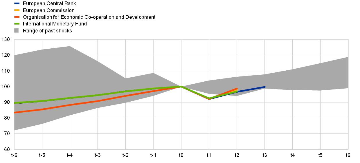
The level of potential output during the COVID-19 crisis depends on what can be considered the full capacity of the economy. When lockdown measures are in effect, the factors of production are still in place, but are prevented from being utilised fully. In this situation, the full capacity of the economy and hence the degree of capacity utilisation and the size of the output gap[3] may be very different from their levels in normal times. Chart 1 illustrates two extreme interpretations for the period in which national lockdowns were imposed and business operations were restricted, as well as when containment measures were subsequently lifted. The first interpretation assumes that the available factors of production are not affected by the lockdown and the related containment measures. For instance, a restaurant still has the same number of tables as before and a car assembly plant the same number of machines. The number of employees available is also unchanged, even if they are, for example, working fewer hours, on short-time working schemes or temporarily absent. Finally, technology does not change significantly in short periods of time and remains available. Under this interpretation, the degree of full capacity is unchanged during the lockdown (see Chart 1, upper panel, blue line). When containment measures are gradually lifted, production factors are fully utilised again (interpretation 1). By contrast, a second interpretation assumes that during the lockdown, none of the resources are available for production (i.e. the restaurant and the plant are closed and the workers need to stay at home). This implies that full capacity collapses to zero in firms that are closed, equivalent to a temporary steep drop in supply and thus in potential output (see Chart 1, upper panel, yellow line). As soon as the lockdown is over and containment measures are gradually being lifted, the degree of full capacity will gradually recover towards its pre-crisis level (interpretation 2).
These interpretations imply very different output gaps as a result of the large fluctuations in the actual level of output during the crisis. In the first interpretation, the output gap becomes negative during the lockdown period (see Chart 1, lower panel, blue line), as actual output falls well below full capacity, which by contrast remains unaffected overall. In the second interpretation, however, the output gap is not affected by the lockdown (see Chart 1, lower panel, yellow line), since actual production is the same as the assumed full capacity. Potential output falls to the same extent as GDP. These two interpretations are of course illustrative extremes and, in practice, the truth lies somewhere in between. This is especially true at the aggregate level, given that the impact of the shock on full capacity has been different across sectors (not least because of differences in the scope for working remotely).
Chart 1
Interpretation of potential output and the output gap
(no units – illustration only)

Source: ECB staff calculations.
3 COVID-19: interplay of supply and demand shocks
The choice of interpretations outlined above determines the degree of cyclicality of potential output in the short term. The more potential output is assumed to be affected by the containment measures, the more potential output will fluctuate in the short term as restrictions are enforced and lifted. The less that is assumed to be case, the steadier potential output will stay. Different empirical approaches can help to establish which interpretation is matched by data, i.e. the degree to which supply, and with it also potential output, has been affected.
Given data limitations, the complex nature of the shock and the interdependence of supply and demand factors, disentangling these factors is a challenging task.[4] As such, changes in the one might affect the other component. In that respect, a recent theoretical study suggests that a supply shock, affecting sectors of the economy asymmetrically, may in turn trigger demand contractions.[5] At the same time, as the great financial crisis showed, demand-side factors may also have persistent or even permanent impacts on potential output.[6]
Empirical analyses, based on limited data, find that both supply and demand dropped after the COVID-19 shock. In the United States, a study was conducted using data on hours worked and wages to estimate labour demand and supply shocks for the aggregate economy and for various sectors. It found that labour supply shocks accounted for a larger share of the fall in hours, although both shocks were noteworthy.[7] Another paper identified the supply and demand shocks from real-time survey data on inflation and real GDP growth and found that in the first quarter of 2020 negative demand had a bigger role in the fall in activity, but in the second quarter reduced supply played a more significant role.[8] Other data and methods suggest that demand factors were stronger and could be explained by uncertainty or fear of infection.[9] Overall, in the United States, empirical studies found that both supply and demand had an important role and, since the nature of the shock was the same across the globe, it can be reasonably assumed that the same holds for the euro area as well.[10]
It was possible for the effects of broader supply-side restrictions to be attenuated in sectors that were able to maintain and adapt production. Production was maintained in sectors that were considered to be essential while, at least in some countries and regions, production was cut back in non-essential sectors. In addition, the degree to which work could be carried out remotely influenced the decline in activity. Empirical papers found that the ability to telework varies greatly across sectors and among workers both in the United States[11] and in Europe[12], and the supply-side effect of the COVID-19 shock has been stronger in sectors where fewer workers were able to carry out their tasks remotely.[13] In addition, negative spillover effects from firms and sectors more affected by social distancing imposed negative externalities on firms not directly affected by social distancing measures, as a result of input-output linkages.[14]
It is not only the degree of fluctuation of potential output in the short term that is difficult to assess, but also the long-term impact of the pandemic. The supply-side effects explored above may be temporary, persistent, or permanent.[15] Empirically, it is not possible to disentangle these effects in real time, which makes it difficult to predict the permanent effects. Nevertheless, one option for trying to gauge the long-term impact is to review the evidence from past exogenous shocks.[16] Box 1 provides some empirical evidence on the effect of selected past exogenous shocks on long-term economic activity.
Box 1 The long-term impact of selected past exogenous shocks on euro area output
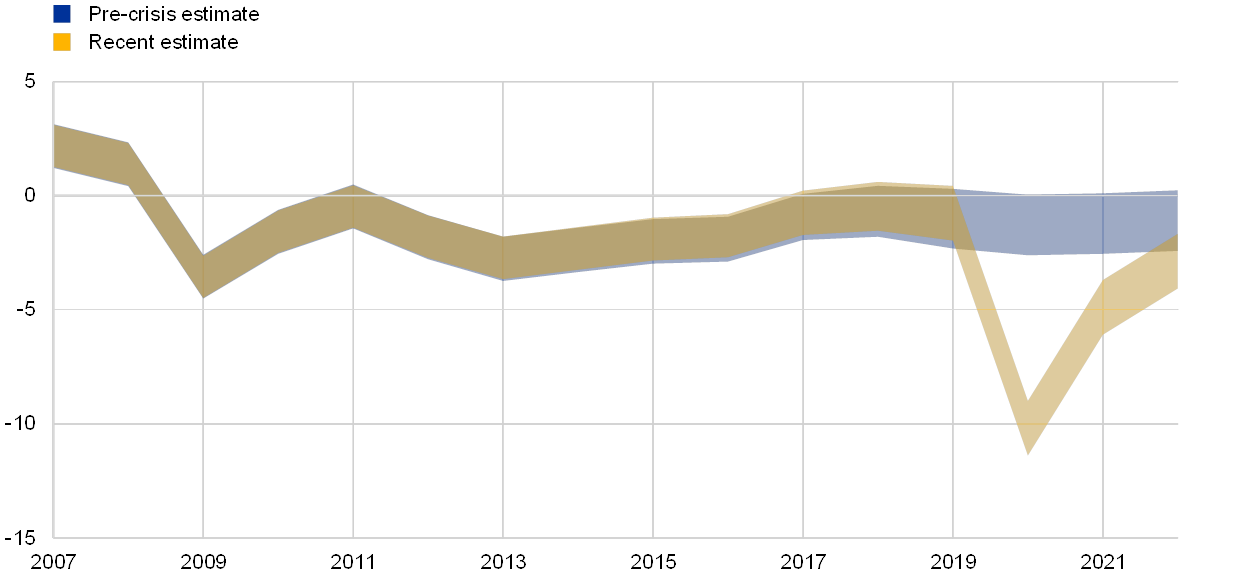
While the COVID-19 shock is unique, previous large exogenous shocks provide a relevant basis for assessing its long-term impact. This box looks at the great influenza pandemic of 1918-19 and the oil price shocks of 1973 and 1979 with the aim of assessing their long-term impact on growth in what are today euro area countries. These episodes can be related to the COVID-19 shock in that they were exogenous, although their severity may have differed (see Chart A). At the same time, the fast, coordinated and large-scale policy response also makes the COVID-19 episode unique.
Chart A
Range of real GDP in past and present exogenous shocks in today’s euro area
(level, year before the shock = 100)
Sources: Maddison Project Database, version 2018; Bolt, Jutta et al., “Rebasing Maddison: new income comparisons and the shape of long-run economic development”, GGDC Research Memorandum No 174, January 2018; June 2020 Eurosystem staff macroeconomic projections; European Commission (EC); International Monetary Fund (IMF); and Organisation for Economic Co-operation and Development (OECD).
Notes: This chart shows GDP for the five years before and after the exogenous shock for an aggregation of the euro area countries. The legend indicates the dates chosen for t0, which is the year before the shock, or, if the shock hit only in the second half of the year, the year of the shock itself. The shocks included in the range include the influenza pandemic in 1918-19, the oil price shocks of 1973 and 1979 and the great financial crisis in 2007-08. The solid lines reflect the latest projections by the international organisations, where t0 is the 2019 level of GDP.
The great influenza pandemic does not appear to have resulted in a statistically significant lasting adverse effect on the GDP growth rate. That pandemic, which propagated worldwide in 1918-19 (namely in the last years of World War I), had a direct impact on labour input. It resulted in high fatality rates in the working age population,[17] absenteeism and shutdowns of businesses. The COVID-19 shock, however, is associated with a much lower fatality rate among the working age population. Moreover, its economic impact is more related to the containment measures aimed at protecting the population and it has resulted in confidence and uncertainty shocks that have affected both households and businesses, with some sectors more affected than others. Estimating a vector error correction model including fatality rate determinants (see below) for the period 1901‑25, we find that the great influenza pandemic had a negative impact on GDP growth. However, the effect on GDP growth is estimated to have been temporary, in contrast to the shock concomitant with World War I.[18]
By contrast, the rises in oil prices of 1973 and 1979 were permanent and had a more lasting effect on euro area GDP growth rates. The oil price shocks largely hit European economies, with productivity being the main channel of economic growth affected.[19] While this shock primarily affected supply, it also had an impact on demand, as income and spending were squeezed in oil-importing countries. The oil price increase was permanent: the level of oil prices never returned to that observed in the early 1970s. Accordingly, we find that the oil price shocks had a permanent negative effect on GDP level and a protracted negative effect on growth rates. The second-to-last column of Table B shows that a permanent 1% increase in oil prices reduced euro area GDP by 0.2% in the long run, regardless of the effect of higher oil prices on capital intensity, which mitigated the negative impact on GDP. Our findings are in line with other papers that link the oil price shocks to the ensuing period of curtailed economic growth.[20]
Our method is based on the estimation of error correction equations, primarily linking the change in GDP to that in capital intensity. Depending on the estimated period, we enhance our estimates with other explanatory factors. For the period of the great influenza pandemic, the equation has the following form:
where, for each country , is the log of annual GDP, the log of capital intensity, the World War I fatality rate and the pandemic fatality rate. Fatality rates are expressed as a percentage of the population. The estimation is carried out using a panel and includes country fixed effects that are not shown in the equation. The coefficient estimates are shown in Table A.
Table A
Error correction model for the period of the great influenza pandemic

Sources: ECB staff calculations; Bergeaud, Antonin et al., “Productivity Trends in Advanced Countries between 1890 and 2012”, Review of Income and Wealth, Vol. 62, No 3, International Association for Research in Income and Wealth, September 2016, pp. 420-444; Barro, Robert J. et al., “The Coronavirus and the Great Influenza Pandemic: Lessons from the ‘Spanish Flu’ for the Coronavirus’s Potential Effects on Mortality and Economic Activity”, NBER Working Paper No 26866, National Bureau of Economic Research, Cambridge, Massachusetts, April 2020.
Notes: The rate of GDP growth, proxied by its log-difference, refers to the annual growth rate of real GDP in US dollar terms adjusted for purchasing power parity in 2010. Capital intensity refers to the ratio of capital to labour expressed in hours worked. Fatality rates are expressed as a percentage of the population. Values for the influenza fatality rate outside of 1918-20 are set to zero. Oil price is expressed in log-level in the long run and in log-difference in the short run. The sample for GDP growth covers 21 countries. Estimation is done by the panel least squares method. The standard errors of the coefficient estimates allow for clustering of the error terms by year. (*), (**) and (***) denote 10%, 5% and 1% significance level respectively.
For the oil price shocks period, the equation has the following form:
where, for each country , is the log of annual GDP, the log of capital intensity and the log of the price of Brent crude oil in euro. The estimation is carried out using a panel and includes country fixed effects that are not shown in the equation. The coefficient estimates are shown in Table B.
Table B
Error correction model for the period of oil price shocks

Sources: ECB staff calculations, Bergeaud et al., op. cit., Barro, Robert J. et al., op. cit.
Notes: The rate of GDP growth, proxied by its log-difference, refers to the annual growth rate of real GDP in US dollar terms adjusted for purchasing power parity in 2010. Capital intensity refers to the ratio of capital to labour expressed in hours worked. Death fatality rates are expressed as a percentage of the population. Values for the influenza death rate outside of 1918-20 are set to zero. Oil price is expressed in log-level in the long run and in log-difference in the short run. The sample for GDP growth covers 21 countries. Estimation is done by the panel least squares method. The standard errors of the coefficient estimates allow for clustering of the error terms by year. (*), (**) and (***) denote 10%, 5% and 1% significance level, respectively.
The COVID-19 shock is expected to be followed by a larger drop in GDP in the euro area than previous exogenous shocks or the great financial crisis. This reflects the large expected short-run effect of the shock, although the uncertainty about the longer run remains high. It should also be noted that in the second half of 2020, a strong rebound in economic activity is expected, which was not the case during the 2007-08 financial crisis. Transferring the results from this box to the current shock, its long-term damage to the economy could be hoped to be rather small should the shock fade out rather quickly (i.e. if a vaccine is found that ensures that the shock is not lasting or recurring).
4 COVID-19: channels of impact on potential output
The coronavirus and, in particular, the related containment and lockdown measures are likely to affect most components of potential output. The channels are discussed below for each component (TFP, capital and labour), also with reference to experience during and after the great financial crisis.
The coronavirus and containment measures negatively affect trend TFP through several channels. Supply chain disruption might be persistent and firms might need to find new suppliers, new transport routes or new locations of production. This might be exacerbated if the current pandemic increases protectionism and accelerates de-globalisation. If this is the case, sectors that have greatly benefited in terms of productivity growth from international exposure and globalisation might experience a decline in trend TFP. Financial distress might increase the financing cost of new, productive projects and might also increase corporate default rates (see Box 2 for a more detailed analysis). The destruction of jobs resulting from a surge in firm exits would potentially lead to productivity losses if reallocation of displaced workers to other firms is slow and results in a deterioration of workers’ skills in the long run.
However, a few factors might counterbalance the negative impact on trend TFP. The COVID-19 shock has had an asymmetric impact on various sectors of activity and might, therefore, result in TFP-enhancing sector reallocation. This may be the case if some low-productivity sectors are more persistently affected and lose economic importance to the benefit of less affected high-productivity sectors. For example, during the great financial crisis, in some countries, notably in Spain and in Italy, trend TFP growth started to improve as the crisis was seen as increasing allocative efficiency by reallocating resources from the low-productive construction sector to the relatively higher-productive manufacturing sector. Moreover, if low-productive firms were relatively more affected by the shock, there could be a “cleansing effect”.[21] Box 2 shows, however, that given the non-economic nature of the COVID-19 shock, there might be less of a silver lining to the present crisis than to the great financial crisis. Finally, although the effect is probably rather small in the short term, containment measures might have accelerated the progress of digital uptake in firms across all sectors and may thus enhance productivity growth in the medium term.[22] Nevertheless, the overall negative impact on trend TFP and its contribution to potential growth might be considerable.
The COVID-19 shock may negatively affect the capital stock in the euro area, mainly through lower investment. First and foremost, despite supportive financing conditions, the high level of uncertainty could adversely affect investment decisions. Furthermore, the decline in value added could also hit investment (accentuated by the “accelerator effect”), while falling corporate margins could dampen investment expenditures.
Capital scrapping and depreciation may be affected by two offsetting effects. Company liquidations might entail some of the capital assets being scrapped before the end of their service life (see also Box 2). On a positive note, the lifespan of existing assets may be extended thanks to less intensive utilisation if they were shut down during the lockdown. The equipment of firms where employees work largely from home might also wear out more slowly, since equipment might be provided by the workers rather than the firm. During the great financial crisis, it seems that the former effect predominated, leading to an increase in the average scrapping rate of capital assets.[23]
The sectors most affected by the decline in activity are also those that contribute the most to changes in the euro area productive capital stock. Traditionally, the manufacturing and retail trade, transport (including travel), accommodation (including hotels) and food and beverage sectors have been the largest contributors to developments in investment in machinery and equipment. The first available data point to a substantial deterioration in investment in 2020, but a rebound in economic activity and investments is expected in the second half of the year. While the contraction in the first half of 2020 could lead to a permanent reallocation of capital from the sectors most affected, the overall impact on potential output depends on how persistently investments are ultimately curtailed.
The labour contribution to potential output could be severely hit but is currently significantly supported by sizeable policy measures. The short-time working schemes introduced in many countries[24] have the potential to limit hysteresis and longer-term scarring in the euro area labour market. However, in the event of a more lasting shock and the eventual scaling down of mitigating policies, hysteresis effects could emerge, resulting in a more persistent increase in the non-accelerating inflation rate of unemployment (NAIRU). This can happen if people become long-term unemployed, which tends primarily to affect the younger and lower skilled. Based on the experience of the great financial crisis, we can assume that the NAIRU will rise again. There are, however, some differences here between that crisis and the present one.
(i) The increase of the NAIRU during the great financial crisis partially reflected the impact of the second phase of the crisis, which was relatively severe.
(ii) The NAIRU is estimated to have declined significantly in recent years, reflecting more flexible labour markets as a result of reforms in several euro area countries. The higher labour market flexibility might reduce the extent to which the NAIRU rises in the face of the current shock.
(iii) In contrast to the present shock, the great financial crisis mostly affected the construction sector and industry, but seemed to be smaller in market services, which have a high weight in the value added of the total economy. The COVID-19 shock, however, is assumed to be affecting all major sectors to a considerable degree and this simultaneous decline may increase the probability of hysteresis effects occurring. In some industrial and market services subsectors, the shock can also trigger or accelerate structural changes. This may imply a larger and more immediate impact on the NAIRU than that seen as a result of the great financial crisis.
If the shock turns out to be more persistent, working age population growth could slow due to lower migration. Immigration has had an upward impact on working age population growth in the euro area recently. Cross-border and immigrant workers tend to work in sectors that are considerably affected by the shock (for example accommodation, retail trade and food service). Due also to a higher share of precarious contracts, they may be more vulnerable to dismissal. In addition, tighter travel restrictions may prevail for an extended period of time and the willingness of workers to move might decrease. This, however, may also cushion the reaction of the NAIRU to the shock in net immigration countries. Due to differences in net immigration, the impact may vary considerably across euro area countries.
Other components of trend labour input might also be affected. The continuation of the recent rise in the trend participation rate may be at risk, for example in the case of older workers withdrawing from the labour market in the aftermath of the shock.[25] Trend participation of women may also be affected as they are more represented in the sectors hit harder by the shock (e.g. accommodation and food service activities; the arts, entertainment and recreation), compared with other sectors less affected.[26] Both groups have made a considerable contribution to the rising trend labour force participation rate in recent decades.
The impact of the shock on components of potential output may depend on which sectors are more affected. The current shock may have a more permanent impact on some service sectors, primarily those that have been relying on the benefits of globalisation – namely accommodation, travel and transportation. But domestic service sectors may also be negatively affected in the longer term. The expansion of services seen in recent decades supported employment growth and likely contributed to the rise of labour supply. An L-shaped shock in these sectors may increase the possibility of declining trend labour input, through the NAIRU, but also potentially through the trend participation rate. In addition, as described above, capital can be negatively affected. In manufacturing, purchases of goods (as opposed to services) can be postponed and pent-up demand may imply stronger growth later. However, at least some subsectors may be permanently affected as the current shock may coincide with the impact of ongoing structural challenges. By contrast, a permanent shock to some manufacturing sectors may increase the probability of a larger shock to capital and TFP components.
Box 2 The impact on potential output of a surge in firm exits as a result of COVID-19
Whether the current crisis will leave long-term scars will depend, among other things, on the number and nature of companies that default as a result of the liquidity strains caused by the lockdown and containment measures. This box uses Orbis and iBACH-sourced financial accounts of firms operating in the private sector of four euro area countries (Germany, Spain, France and Italy) to approximate the number of firms at risk of default as a result of the lockdowns and subsequent weak economic growth. The objective of the analysis is to measure the economic impacts of a surge in firm exits on the drivers of potential output, these being employment, capital and productivity growth.
To gauge the magnitude of the impacts, the analysis simulates the dynamics of the liquidity of firms over time. The sudden collapse in revenues of firms as a result of the lockdowns together with their limited capacity to adjust costs have shocked the liquidity buffers firms have built up over recent years. In order to flag firms facing liquidity shortfalls as a result of the shock[27], it is assumed that the liquidity of firms at any month t is equal to the remaining liquidity from the previous month plus monthly sales net of operating costs.[28] Revenues change according to sector-specific value added consistent with expected headline GDP. The ability of firms to adjust costs, however, depends on estimated elasticities of intermediate and labour expenses to changes in firm-level turnover.[29]
Our analysis shows that Spain is the most affected country, with about 25% of the population of firms with employees at risk of becoming illiquid at the peak of the crisis (28% of employees) assuming no policy support (see Chart A, upper panel, blue bar).[30], [31] The results are in line with or somewhat below other estimates (e.g. those of the European Commission or the OECD).[32] Firms with strong balance sheets, however, could partially weather the losses incurred by relying on working capital buffers. In the light of this, the share of firms running into negative working capital is also computed (see Chart A, upper panel, orange bar). Furthermore, among all those firms under stress, i.e. at risk of either liquidity or working capital shortages, the highly leveraged ones might encounter difficulties in raising external finance to cover temporary shortages and might therefore default.[33] According to this criterion, about three-quarters of the firms identified as encountering liquidity or working capital shortfalls are at risk of exit. They account for 10% to 23% of all firms with employees, and between 10% and 17% of employees in the non-financial business sector (see Chart A, upper panel, dots).
The rapid implementation of policies to support the liquidity of firms has significantly reduced the share of firms under stress as a result of the lockdowns. One of the most effective policies has been the introduction of short-time working schemes, which allow firms to reduce their wage bill by temporarily transferring part of the labour costs to governments. They also keep workers attached to their firms, preserving the valuable worker-firm link. In order to evaluate their effectiveness, it is assumed that firms’ labour costs are reduced in proportion to the share of workers covered by the schemes in each country, which averages 40% of employees. Chart A (upper panel) shows that the short-time working schemes halve the share of firms under liquidity stress in most countries, and reduce by almost two-thirds the employment at risk, given that labour costs account for a large part of firms’ operating costs. These schemes, however, are not as effective in reducing the number of firms at risk of working capital shortfalls. The reason for this is that cash accounts for about 20% of firms’ current assets. The schemes therefore affect a relatively small part of firms’ working capital.
Chart A
Share of firms at risk
Share of firms under stress in a no-policy scenario
(as a percentage of the population of firms with employees)

Source: ECB staff calculations based on Orbis and iBach data.
Share of firms under stress after accounting for the impact of short-time working schemes
(as a percentage of the population of firms with employees)

Chart B (upper panel) shows the total number of employees working in firms at risk of exit, defined as firms with negative working capital and high leverage, in each country as a percentage of the workforce of the non-financial corporation (NFC) sector. It can be seen that under the no-policy scenario, between 10% and 17% of the employees in the NFC sector could lose their job. The share of the NFC capital stock installed in firms at risk of exit is shown in the lower panel. For this exercise, it is assumed that 60% of installed capital can be reused, or in other words 40% of capital is scrapped after firm exit. Under this assumption, up to 7% of the capital stock could be lost as a result of firm exit. Hence the potential costs of firm exit in terms of job separations and capital destruction can be large. The mitigating impact of short-time working schemes is shown by the dots in both panels of Chart B.
Chart B
Employment and capital at risk
(as a percentage of employment in the NFC sector)

Source: ECB staff calculations based on Orbis and iBach data.
The impact of firm exit on aggregate productivity growth is ambiguous. Besides the expected negative impacts of firm exit on TFP growth listed in the main text, the current crisis could have a silver lining for TFP growth. Indeed, sector reallocation triggered by the loss in economic importance of low-productive sectors like those related to tourism and the gain in high-productive ones could increase aggregate TFP growth in the medium term. Furthermore, if low-productive firms are relatively more affected by the shock, there could be a “cleansing effect”. It is possible, however, that the latter will contribute relatively less to aggregate TFP growth than in previous crises. The reason is that the COVID-19 shock is not economic in nature and could therefore affect both productive and unproductive firms in any given sector.[34] Last and most importantly, the acceleration of digital uptake by the corporate sector could result in positive productivity impacts in the medium-term.
To conclude, the large potential economic costs of a surge in firm exits as a result of the COVID-19 shock justify the large support schemes implemented by all European governments. However, if those schemes are withdrawn before the revenues of firms from activity recover, we could see some cliff effects. Hence, to prevent long-term scars from the crisis the design and timing of the exit strategies will be as important as those of the support packages themselves.
5 Quantitative estimates of the impact of COVID-19 on potential output
This section reviews recent estimates of potential output and several statistical methods.
This section presents the unobserved components model (UCM), which is a key tool in the assessment of potential growth within the euro area.[35] The UCM combines a multivariate filter approach with a Cobb-Douglas production function relating potential output to labour, capital and TFP. The underlying model is a backward-looking state-space model that decomposes four key observable variables (real GDP, the unemployment rate, a measure of core inflation and another of wage inflation) into trend and cyclical components. It relies on several economic relationships for this, including a Cobb-Douglas production function, a wage and a price Phillips curve, and an Okun’s law[36] relationship. In the model, a closed output gap is consistent with the absence of excessive price or wage pressures.[37]
At this point in time, modelling potential growth and trend-cycle breakdowns is a challenging exercise. The nature and magnitude of the shock (see Section 2) and its far-reaching implications, especially for the labour market, and extensive government interventions make it necessary to adjust the normal set-up of the UCM. Without being exhaustive, a few aspects that needed to be modified are listed below. First, given the sharp drop in activity in the first half of 2020, the UCM applied to the 1995-2022 period as a whole would lead to a substantial downward revision of potential growth in the period preceding the crisis. To avoid this statistical artefact, potential output estimate is frozen prior to 2020 and is then overlaid with the estimate carried out for the period 2020-22. Moreover, some economic relationships are temporarily affected by the shock, such as the Okun’s law. This relationship had to be adjusted to allow for GDP to fall more than unemployment has risen. Finally, a degree of judgement had to be introduced on certain variables such as the NAIRU or the average number of hours worked so that their trend would better reflect foreseeable medium-term and long-term changes.
Potential growth in the euro area is estimated to have been severely affected throughout the current crisis. Conditional on the Eurosystem staff macroeconomic projections of December 2019, the UCM would originally have suggested that potential output was likely to evolve in line with observations in recent years, between 1% and 2% annually between 2020 and 2022. The COVID-19 crisis has changed the picture, as the latest estimates based on the September 2020 staff macroeconomic projections indicate that potential growth would average between ‑0.3 and 1.1% annually between 2020 and 2022 (see Chart 2, upper panel). Compared with the great financial crisis, the impact is much larger. In the wake of the previous crisis, potential growth only fell by somewhere between 0.0% and 0.7% per year. Potential output would, however, fall less than real GDP, resulting in an unprecedented drop in the output gap (see Chart 2, lower panel).
Chart 2
Euro area potential growth and output gap
Potential growth
(annual percentage change)

Source: ECB staff calculations.
Notes: Shaded areas indicate interval estimates based on the UCM (representing an uncertainty band of plus/minus two standard deviations around the point estimate). The blue area represents the UCM projection conditional on the December 2019 Eurosystem staff projections, while the yellow area represents the UCM projection conditional on the September 2020 ECB staff projections.
Output gap
(percentage of potential output)
The level of euro area potential output would remain well below the path suggested by pre-crisis projections. This can be illustrated with the cumulative loss of potential output estimated with the UCM between December 2019 and September 2020 (see Chart 3). Overall, the loss in the level of potential output would reach almost 3% by the end of 2022. Even though potential growth would return fairly soon to pre-crisis rates, the potential output level would be affected for longer. The UCM provides a tentative outlook on the future level of potential output. The projection falls between that of the IMF and that of the European Commission. Nevertheless, all these estimates are subject to considerable uncertainty, as indicated by the shaded areas in the charts above, accounting for a range between estimations of 95%. Furthermore, caution is warranted when using such gaps as a proxy for the impact of the crisis. Real-time estimates of potential output are often subject to substantial revisions, especially in times of crisis, and estimates of the euro area aggregate mask significant heterogeneity across individual euro area countries.
Chart 3
Loss in euro area potential output
(percentage)

Sources: ECB staff calculations, IMF World Economic Outlook, European Commission.
Note: This chart shows the difference in the level of potential output before the crisis levels and based on the most recent estimates.
According to the UCM, the contribution of labour is pivotal to the changes in potential output. The contribution of labour to potential growth can be traced back to trends in the working age population, the labour force, the unemployment rate and hours worked per employee. Estimates of the UCM show that the latter two components would see their trend affected most by the current crisis. The NAIRU would rise significantly and remain elevated even in 2022 due to hysteresis phenomena. However, this effect might be mitigated by short-time working schemes, which is not fully captured by the UCM. Trend average hours worked would weigh on potential growth until the end of 2021 before having a positive effect in 2022. More incidentally, capital stock would also contribute to the downward revision of potential growth linked to the fall in investment (see Box 2 for an analysis of the balance sheets of companies). Conversely, revisions to TFP growth would have a relatively small effect on potential growth. This can be explained by the difficulty faced by the model in capturing major shifts that would affect potential: reallocation of resources, accelerated development of teleworking, increased spending on research and development or biotech, etc. (see Chart 4).
Chart 4
Revisions of components of potential output growth due to the COVID-19 crisis
(annual percentage point difference)
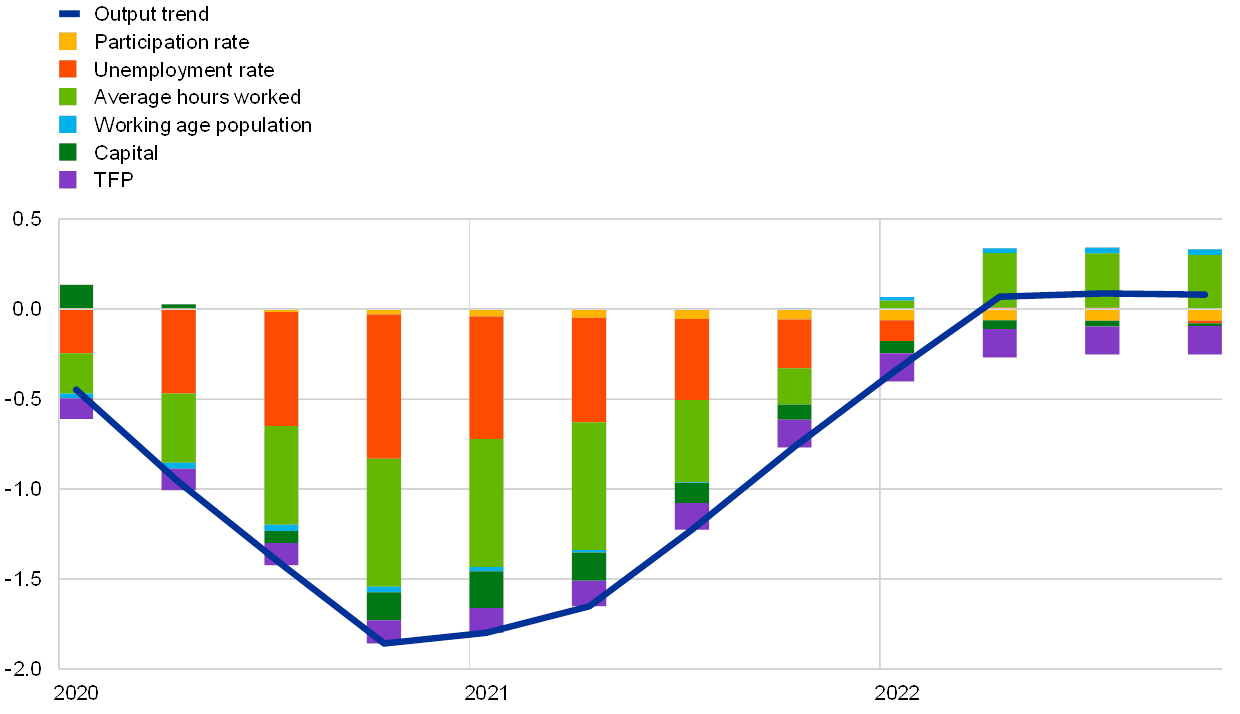
Source: ECB staff calculations.
Note: This chart shows the difference in the breakdown of potential output growth components before the crisis and based on the most recent estimates.
Box 3 A range of quantitative estimates of the impact on potential output
Different statistical methods can be used to estimate potential output. The methods presented in this box cover simple statistical filters (Hodrick-Prescott, Beveridge-Nelson), a small multivariate filter (a survey-based measure of slack[38]), the Blanchard-Quah structural vector autoregressive (SVAR) model (using an unemployment rate augmented by people under short-time working schemes), the unobserved components model discussed in detail above, and the Jarociński-Lenza model.[39]
The mean of estimates provided by six different methods shows potential growth stalling and a significantly negative output gap (see Chart A). Most estimates show lower, but still positive, potential growth in 2020, and as a consequence, a significant negative output gap, of at least -3.5% in 2020. One exception is the Jarociński-Lenza model, which estimates a significant drop in potential output and a more stable, albeit negative, output gap.[40]
Overall, the quantitative estimates fall in between the two extreme interpretations introduced in Section 1, confirming that euro area potential output has been seriously affected by COVID-19, but to a lesser extent than real GDP.
The uncertainty currently surrounding potential output and output gap estimates is at a high level. The range of estimates introduced here becomes extremely wide in the second quarter of 2020: the average width of the range of potential growth is about 2 percentage points, increasing to about 5-7 percentage points during the great financial crisis, and to 16 percentage points in the second quarter of 2020. The range declines beyond the second quarter of 2020 mostly because two of the six measures (the Jarociński-Lenza model and the survey-based measure of slack) do not use forecast data and therefore are not available between the third quarter of 2020 and the final quarter of 2022.
However, the large drop in the output gap may reflect an overestimation of the downward pressures on inflation. This reflects important government support measures for firms and households. Disposable income of households fell less than GDP in the first half of 2020, and thus the cyclical component of disposable income might be less negative than the output gap. As a consequence, the output gap might overestimate downward inflationary pressures. Likewise, labour market slack measures, such as the unemployment gap, defined as the difference between the unemployment rate and the NAIRU, might not be the most adequate measure of inflationary pressures on wages either. Owing to short-time working schemes, the headline unemployment rate has increased less than the business cycle would have suggested. As a result, the unemployment gap may understate downward wage pressures.
Chart A
Euro area potential growth and output gap
(upper panel: annual percentage change; lower panel: percentage of potential output)

Source: ECB staff calculations.
Notes: The range contains six indicators up to the second quarter of 2020, namely the Hodrick-Prescott and Beveridge-Nelson filters, the SVAR model of Blanchard-Quah, the survey-based measure of slack, the UCM and the Jarociński-Lenza model, and only four measures after that (as the survey-based measure and the Jarociński-Lenza model are unavailable). The second quarter of 2020 is marked with a blue circle.
6 Conclusions
The COVID-19 pandemic and related containment measures affect the industries and countries of the euro area to an extent that is likely to affect potential output. However, the scale of this impact over the short and long term is highly uncertain. For the short term, the amplitude of the fluctuation depends significantly on how containment measures are assumed to affect potential output. In the long run, it depends on how long the pandemic will last and the extent to which policy measures are able to protect the economy from excessive scarring, among other factors.
The current crisis is likely to induce some structural changes in the euro area economy and economic policies will play a pivotal role in facilitating this change. In particular, they have an important role in protecting the firms and employees of shrinking industries from hysteresis. Thus far, ECB analysis shows that the rapid implementation of short-time working schemes across European countries has mitigated the potential permanent employment losses resulting from lockdowns.[41] State-backed loans have also been key to facilitating firms’ access to liquidity to cover working capital shortfalls. Such measures are crucial to protect the euro area economy from long-term scarring.
- See the article entitled “Potential output in the post-crisis period”, Economic Bulletin, Issue 7, ECB, 2018.
- Potential output estimates are often procyclical and reflect developments in demand conditions. On the one hand, this procyclicality could partly be a statistical artefact due to methodological issues, such as the well-known end-point problem of filtering procedures. On the other hand, it could also reflect business cycle fluctuations, for example in investments in physical capital, or in research and development and innovation, leading to procyclical estimates of the capital stock and trend TFP growth.
- Normally, capacity utilisation represents the output gap well: “capacity utilisation is usually defined as the ratio of actual output to some measure of potential output” (see Nelson, Randy A., “On the Measurement of Capacity Utilization”, The Journal of Industrial Economics, Vol. 37, No 3, Wiley, March 1989, pp. 273-286). It follows that full capacity of the economy corresponds to potential output.
- Barry Eichengreen said “As someone who's estimated lots of models designed to distinguish supply and demand shocks, good luck identifying them” (see Vaitilingam, Romesh, Likelihood of a coronavirus recession: Views of leading US and European economists, , VOX, Centre for Economic Policy Research Policy Portal, 14 March 2020.
- See Guerrieri, Veronica et al., “Macroeconomic Implications of COVID-19: Can Negative Supply Shocks Cause Demand Shortages?”, NBER Working Paper No 26918, National Bureau of Economic Research, Cambridge, Massachusetts, April 2020.
- See the article entitled “Potential output in the post-crisis period”, Economic Bulletin, Issue 7, ECB, 2018.
- See Brinca, Pedro et al., “Measuring Labor Supply and Demand Shocks during COVID-19”, Working Paper 2020-011, Federal Reserve Bank of St. Louis, St. Louis, Missouri, October 2020.
- See Geert, Bekaert et al., “Aggregate Demand and Aggregate Supply Effects of COVID-19: A Real-time Analysis”, Finance and Economics Discussion Series 2020-049, Federal Reserve Board, Washington D.C., 26 May 2020.
- See Goolsbee, Austan and Syverson, Chad, “Fear, Lockdown, and Diversion: Comparing Drivers of Pandemic Economic Decline 2020”, NBER Working Paper No 27432, National Bureau of Economic Research, Cambridge, Massachusetts, June 2020.
- Two studies confirm this. See Balleer, Almut et al., “Demand or Supply? Price Adjustment during the Covid-19 Pandemic”, CESifo Working Paper No 8394, Munich Society for the Promotion of Economic Research – CESifo, GmbH, Munich, August 2020 and Boham, D.A.R. and Smadu, A.I., “Was COVID‑19 a supply or a demand shock? Evidence for Dutch sectors”, mimeo, 2020.
- See Papanikolaou, Dimitris and Schmidt, Lawrence D.W. “Working Remotely and the Supply-side Impact of Covid-19”, NBER Working Paper No 27330, National Bureau of Economic Research, June 2020 and del Rio-Chanona, R. Maria et al., “Predicting the supply and demand shocks of the COVID-19 pandemic: An industry and occupation perspective”, VOX, Centre for Economic Policy Research Policy Portal, 16 May 2020
- See Barrot, Jean-Noël et al., “Sectoral effects of social distancing”, Covid Economics, Vetted and Real-Time Papers, No 3, Centre for Economic Policy Research, 10 April 2020, pp. 85-102.
- After the initial shock, some changes in the way we work might be expected. For example, according to estimates, in the United States, nearly 40% of jobs could be plausibly performed from home. See Dingel, Jonathan and Neiman, Brent, “How many jobs can be done at home?”, Covid Economics, Vetted and Real-Time Papers, No 1, Centre for Economic Policy Research, 3 April 2020, pp.16-24.
- See Laeven, Luc, “Pandemics, Intermediate Goods, and Corporate Valuation”, CEPR Discussion Paper DP15022, Centre for Economic Policy Research, 9 July 2020.
- Possible permanent impacts are discussed in Cerra, Valerie et al., “Hysteresis and Business Cycles”, IMF Working Paper WP/20/73, International Monetary Fund, May 2020.
- See Ludvigson, Sydney C. et al., “COVID-19 and The Macroeconomic Effects of Costly Disasters”, NBER Working Paper No 26987, National Bureau of Economic Research, Cambridge, Massachusetts, September 2020 and Jordà, Òscar et al., “Longer-run Economic Consequences of Pandemics”, NBER Working Paper No 26934, National Bureau of Economic Research, Cambridge, Massachusetts, April 2020.
- The death toll estimates range from 50 million to close to 100 million, representing 2.5% to 5% of the world’s population (see Maddison Historical Statistics, 2020 and Cirillo, Pasquale and Taleb, Nassim Nicholas, “Tail risk of contagious diseases”, Nature Physics, Vol. 16, Nature Research, 25 May 2020, pp. 606-613.
- This outcome is consistent with Barro, Robert J. et al., “The Coronavirus and the Great Influenza Pandemic: Lessons from the ‘Spanish Flu’ for the Coronavirus’s Potential Effects on Mortality and Economic Activity”, NBER Working Paper No 26866, National Bureau of Economic Research, Cambridge, Massachusetts, April 2020.
- The price of a barrel of Brent oil rose by 168% in 1974, followed by a rise of 51% in 1979 and 67% in 1980. The shock was triggered by political events affecting the main producing countries.
- Blinder, Alan S. and Rudd, Jeremy B., “The Supply-Shock Explanation of the Great Stagflation Revisited”, in Bordo, Michael D. and Orphanides, Athanasios (eds.), The Great Inflation: The Rebirth of Modern Central Banking, University of Chicago Press, Cambridge, Massachusetts, June 2013, pp. 119-175.
- See Caballero, Ricardo J., and Hammour, Mohamad L., “The Cleansing Effect of Recessions”, The American Economic Review, Vol. 84, No 5, December 1994, pp. 1350-1368.
- The OECD has estimated that a 10 percentage point increase in the adoption of high-speed broadband (or cloud computing) would translate into a contemporaneous increase in TFP growth of 1.4 percentage points (see Gal, Peter et al., “Digitalisation and productivity: In search of the holy grail – Firm-level empirical evidence from EU countries”, OECD Economics Department Working Papers No 1533, OECD Publishing, Paris, 12 February 2019.
- See Anderton, Robert et al., “Potential output from a euro area perspective”, ECB Occasional Paper Series, No 156, ECB, November 2014.
- See the box entitled “Short-time work schemes and their effects on wages and disposable income”, Economic Bulletin, Issue 4, ECB, 2020
- See the article entitled “Drivers of rising labour force participation – the role of pension reforms”, Economic Bulletin, Issue 5, ECB, 2020.
- Adams, Abigail et al., “Furloughing”, CEPR Discussion Paper DP15194, Centre for Economic Policy Research, August 2020.
- Hence the analysis accounts only for firms that were liquid before the COVID-19 crisis.
- Following Schivardi, Fabiano and Romano, Guido “A simple method to estimate firms’ liquidity needs during the Covid-19 crisis with an application to Italy”, Covid Economics, Vetted and Real-Time Papers, No 35, Centre for Economic Policy Research, 7 July 2020, pp. 51-69.
- Initial liquidity is approximated by the liquidity level of firms at the latest available year, 2017 in the case of this exercise, and monthly sales and costs are computed simply as annual sales or costs divided by 12. Finally, firm-level data are weighted so they are representative of the population of firms in each country.
- If the analysis also took into account corporations with no employees and sole traders, the share of firms at risk of illiquidity would go up in all countries by about 5 percentage points. If the original analysis included firms that were illiquid at the start of the crisis, the share of illiquid firms at its peak could double in all countries.
- The severe impact of the crisis on Spain, and to a lesser extent on Italy, is grounded in its sector composition and the dominance of micro firms in the productive structure.
- The most similar study, although with better Italian data, is Schivardi and Romano, op. cit., who estimate that about 20% of firms in Italy might be at risk. The European Commission estimates that 35% of firms across the EU27 would be under liquidity stress in their intermediate scenario, whereas the OECD estimates that about 30% of firms would be at risk of illiquidity after two months of lockdown.
- Firms in the top 25% of the country-sector distribution of leverage are assumed to be “highly leveraged”.
- ECB internal work confirms that whereas the average productivity of firms at risk of exit in Spain and Italy is clearly lower than that of other firms, this is not the case in Germany and France. In the latter two countries the productivity of firms at risk of exit is similar to that of less vulnerable firms, even after controlling for sector of activity. This is different from other crises, in which exiting firms were significantly less productive than incumbents.
- The estimates presented in this section are conditional on the September 2020 ECB staff projections.
- Okun’s law links cyclical unemployment to the output gap.
- The UCM approach estimates the trends of the different production function inputs jointly in a system of equations in which the trend-cycle decomposition is subject to certain key, albeit reduced-form, economic relationships. For further explanation, see Tóth, M., “An Unobserved Components Model to Estimate Potential Output in the Euro Area – a Production Function Based Approach”, ECB Working Paper Series, ECB (forthcoming).
- See the box entitled “A survey-based measure of slack for the euro area”, Economic Bulletin, Issue 6, ECB, 2015.
- Jarociński, Marek and Lenza, Michele, “An Inflation-Predicting Measure of the Output Gap in the Euro Area”, Journal of Money, Credit and Banking, Vol. 50, No 6, 21 May 2018 pp. 1189-1224.
- Nevertheless, in that model, the output gap estimate is significantly determined by the conditioning on inflation the model prescribes.
- See also the box entitled “Short-time work schemes and their effects on wages and disposable income” Economic Bulletin, Issue 4, ECB, 2020.