
Inequality and macroeconomic policies
Intervention by Vítor Constâncio, Vice-President of the ECB, at the Annual Congress of the European Economic Association Lisbon, 22 August 2017
Ladies and gentlemen,
It is indeed a pleasure to participate in this timely discussion on the distributional impact of macroeconomic policies. For too long, the distribution of income and wealth was almost ignored by macroeconomics. As recently recalled by Krusell, this is perhaps due to the “presumption in the literature that the distribution does not matter in the determination of aggregates”.[1] In the 1990s, some studies underlined the end of the Kuznets’ phase of declining inequality and demonstrated that the trade-off between equality and growth no longer seemed to hold empirically.[2] The analysis of distribution in macro theory was however not pursued. A possible second reason for the neglect, could have been that income distribution was not a macroeconomic concern, as it was mostly explained by micro factor price theory with the consequence that at the macro level, “trickle-down economics” would be the right approach to economic policy.
These views were wrong and, naturally, the crisis shattered both presumptions.
First, the contributions of Mian and Sufi, Carroll or Muellbauer[3] showed how relevant heterogeneities related to indebtedness, credit restrictions or marginal propensities to consume out of different sources of income or wealth, were important to explain aggregate consumption behaviour before and after the crisis. Since then, the Heterogeneous Agents New Keynesian – HANK – class of models became an active area of research on the monetary policy transmission mechanism.[4] The recent contribution of Ahn, Kaplan, Moll, Winberry and Wolf (2017) at the NBER Macroeconomics Annual Conference[5] titled “When inequality matters for Macro and Macro matters for inequality” demonstrates how significant the feedback loop is and how models with realistic household heterogeneity better fit empirical consumption dynamics.
Second, the social and political aftermath of the crisis have shown how important distribution of income and wealth as an economic policy issue is. In this respect, the seminal empirical and policy contributions of Atkinson, Piketty, Saez, Milanovic and others, were very relevant to make the point as they analysed the dynamics of the distributions of household income and wealth, across many countries and over many decades. The shocking increase of inequality since the late seventies and the hollowing out of the middle class in many advanced economies, as showed in the famous “elephant graph” of Milanovic,[6] have focused minds on developments in inequality. The striking developments can be seen in Table 1 from Alvaredo et al. (2017).[7]
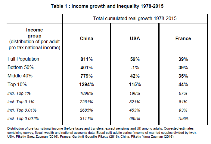
Source: Alvaredo, F., L. Chancel, T. Piketty, E. Saez, and G. Zucman (2017), “Global inequality dynamics: new findings from WID.world”, NBER Working Paper 23119.
The data for the US from 1978 to 2015 show a cumulated decrease of 1% in the income of the bottom 50% of the population whereas the top 10% saw their income increase by 115% and the top 1% by 198%, a segment of the population that, by 2015, owned 20% of income and 40% of total US wealth.
The numbers for France are significantly less unbalanced. In general, developments of inequality within European countries have been more subdued in recent decades than in other parts of the world. Chart 1 shows this well, by depicting the evolution of income inequality, measured by the Gini coefficient on household disposable income.[8]
Chart 1: Income inequality over time, Gini coefficient (1970-2015)
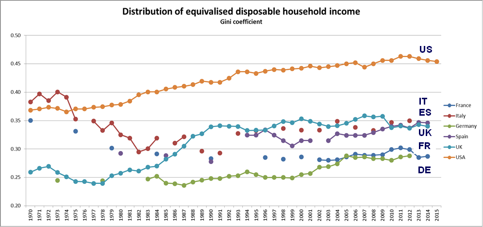
Source: The Chartbook of Economic Inequality, https://www.chartbookofeconomicinequality.com.
Note: The chart shows the evolution of the Gini coefficients on household disposable income. The series for Italy is "Per capita income" and that of the USA "Equivalised gross household income".
The first key fact shown in the chart is that, while income inequality has been steadily rising since the 1970s in the US and the UK, it has been quite stable in continental Europe or even declining as in France and Italy. In particular since the 1990s, the Gini coefficient has been relatively stable in the European countries.
Equally important, the chart documents that the bulk of the dynamics in inequality is driven by low-frequency developments driven by structural and institutional factors, rather than by shocks at the business-cycle frequency.
Chart 1 uses disposable income which hides the much higher inequality associated with the distribution of income before taxes and transfers. To illustrate this point, Chart 2 from Wang and Caminada (2014)[9] shows that difference and the fact that the fiscal systems of European countries dampen income inequality substantially more than those in other countries: in Europe, the difference between the Gini coefficient on market (gross) and disposable (net) income is almost 20 percentage points, more than twice the difference in other countries.
Chart 2: Fiscal redistribution of income in the EU and other countries
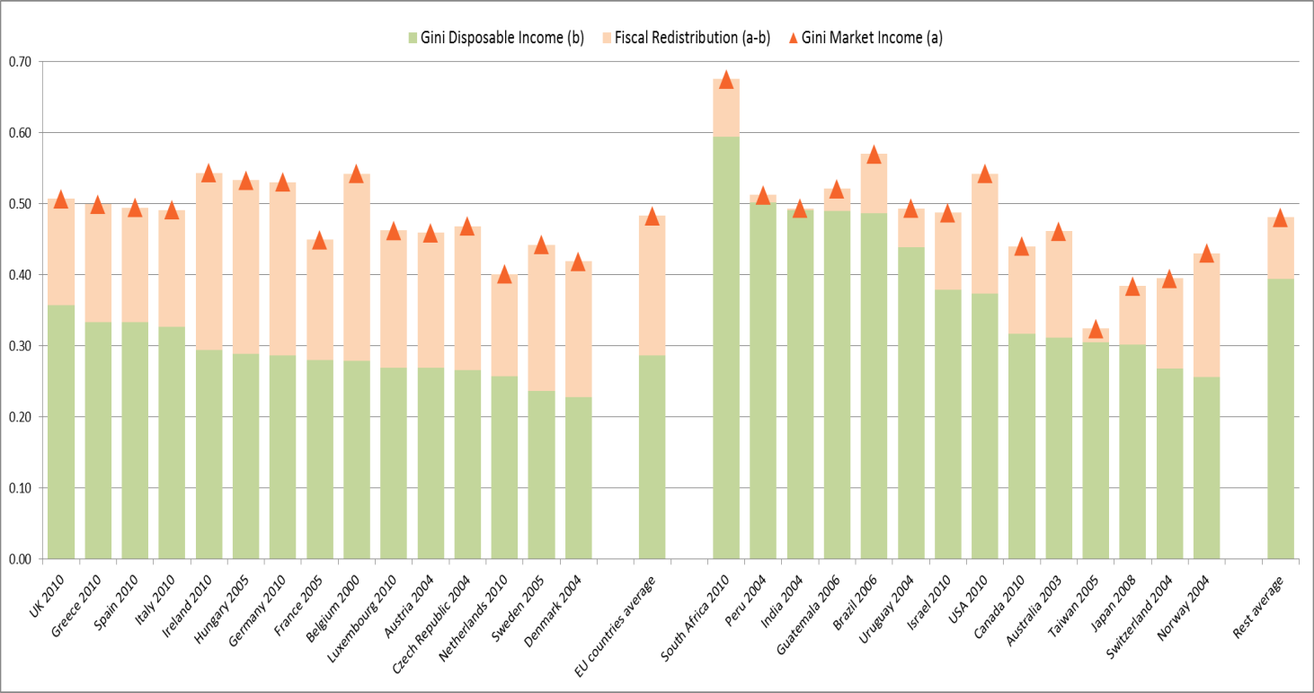
Source: Caminada and Wang (2014).
Note: The chart shows the extent of the fiscal redistribution as given by the difference between the Gini coefficients on market (gross) income and disposable (net) income.
The slow-moving nature of inequality is also confirmed with the more recent survey data from the Eurosystem Household Finance and Consumption Survey (HFCS). Chart 3 summarises the euro area distributions of household income and net wealth[10] since 2010.
Chart 3: Income and net wealth inequality in the euro area
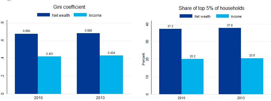
Source: Eurosystem Household Finance and Consumption Survey, waves 1 and 2.
Note: The chart shows gross household income and net wealth per household, defined as the sum of total assets net of total liabilities
Both the distribution of income and the distribution of household net wealth remained stable. For example, the Gini coefficient on net wealth increased only modestly, from 68.0% in 2010 to 68.5% in 2013. Similarly, the share of the top 5% of households on total net wealth remained between 37% and 38%.
Based on the evidence mentioned above, one could already draw some tentative implications for monetary policy. First, given the slow-moving nature of inequality, one could argue that the prevailing monetary policy regime, defining long term goals, is likely to be the most important factor through which central banks may influence the distribution of income and wealth. For example, the conquest of inflation in countries going through prolonged experiences of high inflation is arguably an important factor contributing to the reduction in inequality.
The second tentative implication is that, for a given monetary policy framework committed to a low inflation regime, the specific measures adopted to respond to cyclical developments are unlikely to significantly alter inequality.
It is useful to bear in mind these considerations when discussing a topic that has recently received much attention in the public debate, i.e. how non-standard monetary policies, such as those undertaken in the recent years by the European Central Bank, affect the welfare of individual households. More specifically, to what extent non-standard monetary policies affect wealth inequality and income inequality in the short- and medium run? Which households benefit from those policies and how much?
Despite the two tentative conclusions above, I do not intend to simply brush aside this debate. Indeed, while measures such as the top shares and Gini coefficients are important to consider when thinking about inequality, they can sometimes mask specific dimensions of household heterogeneity, such as those along demographic or socioeconomic characteristics, which can be investigated in data from household surveys (containing additional information beyond the data on income). For example, it is possible to analyse to what extent not only the Gini coefficients, but also income and wealth of individual households react to changes in the unemployment rate or to increased growth of wages and asset prices.[11]
Let me provide some new empirical evidence on this topic based on ongoing work at the ECB by Lenza and Slacalek.[12] More specifically, they quantified how the ECB’s recent Asset Purchase Programmes (APP) affected the income and wealth of individual households in the four largest euro area countries, combining aggregate and household-level data.
First, they estimate the effects of the ECB’s unconventional monetary policy on components of household income and wealth using a Bayesian vector autoregression (VAR) which includes variables that affect wealth – house and stock prices – and variables that affect income – the unemployment rate and wages.[13]
The APP shock is identified by assuming (i) that it affects the term-spread on impact, without leading to a change in standard monetary policy over the full sample[14] under analysis (which spans three years) and (ii) that it has a positive effect on the real economy, on impact.[15] The shock is scaled to a term-spread reduction by 34 basis points, which is the estimated level of the impact of the announcement of the December 2016 APP package on the euro area 10-year bond rates. This implies that the size of the impact considered in the estimates presented in the charts below is smaller than the total effect of our unconventional policies from 2014 to 2016. The analysis is nevertheless representative and conclusive regarding the distributional impact of our monetary policy.
The VAR estimated for the four largest euro area countries shows a degree of heterogeneity across the countries that can be taken as representative of the dispersion that would be found in all other euro area countries (see Chart 4).
Chart 4: Effects of ECB’s Asset Purchase Programme on household income and wealth components
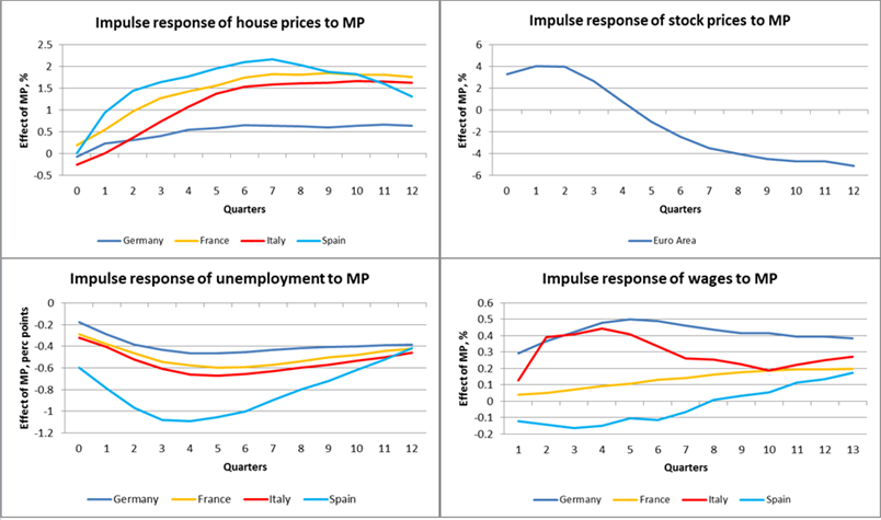
Source: ECB calculations.
Chart 5 below shows the four countries’ average reaction to the relevant variables (house and stock prices, unemployment and wages), four quarters after the impact of the APP shock.[16]
Chart 5: Effects of ECB’s Asset Purchase Programmes on asset prices and macroeconomic variables
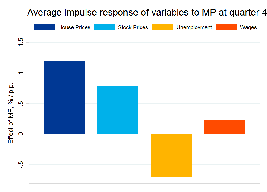
Source: ECB calculations.
Note: The chart shows estimated VAR impulse responses 4 quarters after the impact of the Asset Purchase Programmes (APP) shock. The bars show average responses across the 4 big euro area countries (DE, ES, FR, IT). Responses are shown in percent for house prices, stock prices and wages; in percentage points for unemployment.
The APP purchases are estimated to increase house prices by more than 1% and stock prices by 0.8%. As for the variables, which affect household income (in the bottom two panels): the unemployment rate declines by roughly 0.7 percentage points, while wages rise somewhat.[17]
In the second step, these aggregate results are combined with household-level data to estimate the effects of monetary policy on individual households. The HFCS provides detailed household-level data on income and wealth, but so far only for two waves. However, since the bulk of the effect on wealth occurs via asset prices, we can assume that the response of individual wealth components to the APP after four quarters mirrors the response of asset prices at that horizon.[18] The assumption seems acceptable given the short horizon we are considering and given the empirical evidence on the sluggishness of adjustment of holdings of real and also financial assets in household portfolios.[19]
As for net wealth, Chart 6 shows that the effects of the APP on household wealth are very modest across its distribution:
Chart 6: Effects of Asset Purchase Programs on the wealth distribution
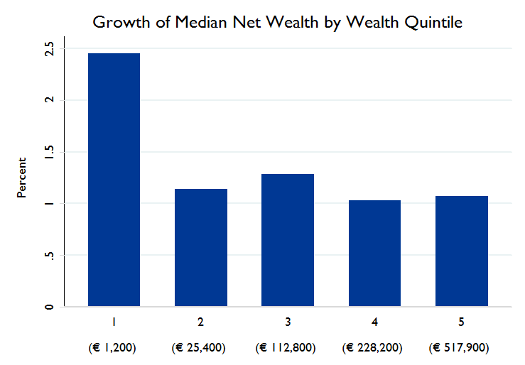
Source: ECB calculations, Eurosystem Household Finance and Consumption Survey.
Note: The numbers in brackets show initial median net wealth levels. Euro area aggregates are calculated as the total for the four large countries: Germany, Spain, France and Italy.
Most quintiles increase by around 1%. The median net wealth in the lowest quintile increases by 2.5% from a rather low level, from EUR 1120 to EUR 1150 and can in part be driven by the leverage of the households Similarly, the Gini coefficient on net wealth barely changes – it ticks down from 68.09 to 68.07.[20]
These results appear to be fully in line with my previous considerations based on the long-run evolution of inequality measures.
Another way of illustrating why the effect of APP on wealth distribution does not seem to have been significant is provided by the analysis in Adam and Tzamourani (2015).[21] They use the euro area average wealth composition by asset classes taken from the HFCS, and simulate the effects on the wealth distribution of an arbitrary increase of 10% in the prices of each asset class: housing, equities and bonds. The results are shown on Chart 7, taken from their paper.
Chart 7: Capital gains across Euro Area net wealth groups
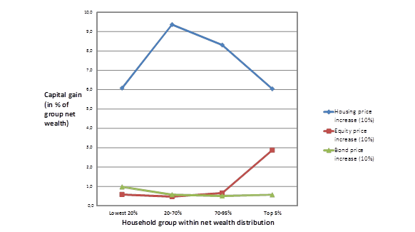
Source: Adam, K. and P. Tzamourani (2016): "Distributional consequences of asset price inflation in the euro area", European Economic Review.
The chart shows that the effect of housing prices on wealth dominates the impact both of equities or bonds. It also illustrates that changes in housing prices reduce inequality in wealth distribution. Bond price increases are fairly neutral and equity price variations aggravate inequality but their effect is smaller than the one from housing prices, at the euro area level.
The overall effect of APP on wealth distribution in the four countries analysed for the recent period in Chart 6 should therefore not come as a surprise.
Let me now discuss how the effects of APP on income of individual households are estimated. The impulse responses give information about the aggregate response of the intensive (wages) and the extensive (unemployment) margin.
To distribute the decline in the unemployment rate across households depending on their demographics (such as age, education, marital status and the number of children), a probit model is estimated at the country level with the employment status as the dependent variable.[22] Such a model captures some heterogeneity in the probability of employment across households. The fitted values from the probit model are then used to run a simulation that distributes the aggregate decline in unemployment across households.[23] Chart 8 compares the changes in the unemployment rates across income quintiles.
Chart 8: Effects of Asset Purchase Programs on employment
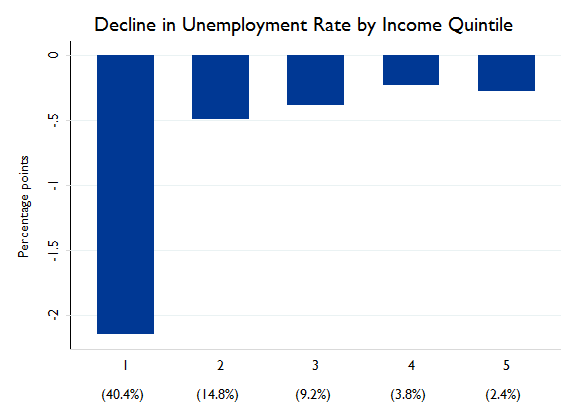
Source: ECB calculations, Eurosystem Household Finance and Consumption Survey.
Note: The numbers in brackets show initial unemployment levels in percent. Euro area aggregates are calculated as the total for the four large countries: Germany, Spain, France and Italy.
The key point to note is that households with lower income are at any point in time substantially more likely to be unemployed and that their employment status also tends to react more significantly to monetary policy impulses. The aggregate decline in unemployment following the APP disproportionately impacts groups with a higher share of the unemployed, such as those in the lowest income quintile.[24] The effect is economically important as in that quintile unemployment rates drop by more than 2 percentage points. For the remaining income quintiles the drop in the unemployment rates does not exceed 0.5 percentage points.
These changes in the employment status affect the distribution of income and, overall, tend to compress income inequality.[25] This result confirms that, from the distributional perspective, the main impact of expansionary monetary policies is on the reduction of unemployment with positive effects on the reduction of inequality.
The positive overall effect of unemployment reductions and wage increases on the income distribution is shown on Chart 9. The mean income in the lowest quintile increases by almost 3.5%, which is substantially higher than the impact in the rest of the distribution. These changes have effects on the income distribution with the Gini coefficient on income declining from 43.1 to 42.8.
Chart 9: Effects of Asset Purchase Programs on the income distribution
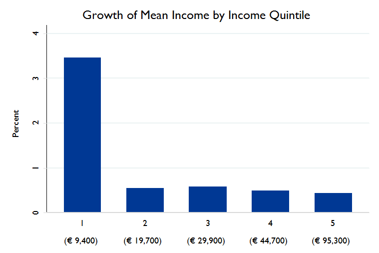
Source: ECB calculations, Eurosystem Household Finance and Consumption Survey.
Note: The numbers in brackets show initial household income levels. Euro area aggregates are calculated as the total for the four large countries: Germany, Spain, France and Italy.
In conclusion, let me summarise these findings in two main points.
First, the effects of monetary policy on aggregate measures of inequality, such as the Gini coefficient are rather modest, compared to the low-frequency dynamics of these indicators over the past several decades. This is more the case for household wealth than for income. In particular, non-standard monetary policy measures can have substantial income (and employment) effects for subgroups of households such as the unemployed. Those measures can improve their welfare and contribute toward reducing income disparities, at least in the short-term.
Second, the low-frequency dynamics in inequality is more likely affected by structural and institutional factors, such as skill-biased technological progress, economic globalisation and changes in the progressivity of fiscal systems. In this context, those drivers may very well aggravate the situation as a result of further technological developments in artificial intelligence and robotisation. The hollowing out of the middle class and the increasing polarisation of incomes in the labour market will presumably continue unabated. Education promotion or the introduction of a Universal Basic Income (UBI) will not change that trend. According to the OECD the UBI could even aggravate poverty.[26]
The Kuznets’ hypothesis[27], stating that as development progresses inequality first increases and then starts decreasing as income grows, was confirmed until the 1970s with inequality decreasing since the period before World War I. The increase of inequality since the 1970s however, has disproved the hypothesis. A subsequent Kuznets’ inequality decline phase, with the same causes of the first (higher taxes and transfers, wars, revolutions, hyperinflation and nationalisations) seems quite unlikely at present. On the other hand, according to Atkinson, Piketty or Milanovic, effective changes would require interventions at the level of market results by operating changes in endowments, which seem unlikely to happen. Indeed, the type of measures they refer to could include wealth taxes, meaningful inheritance taxes, Employee Share Ownership Plans (ESOPs) and share distributions[28], birth endowments in the form of financial assets, for example.[29] Most of these are seen by many economists as distortions detrimental to economic efficiency. Usually, this concept refers to potential Pareto improvements occurring when the income winners could compensate the losers, even if they do not do it. These are usually referred to as “welfare enhancing” consequences which, obviously, do not include any considerations about distribution while pretend to be the basis of “scientific” economic advice.
Maybe the normative word “welfare” in this narrow sense is an ambiguous misnomer that we should no longer use. This does not imply that economists should stop giving advice on economic efficiency and growth which are of course essential to reduce poverty and inequality. At the same time, we should be aware that all policies involve trade-offs and have distributional consequences, which are often forgotten or concealed. That is why Gunnar Myrdal underlined that economics could hardly be value neutral: He proposed that the only acceptable approach was for a researcher to disclose his values not hiding a pretense of science.[30] On this point, at the American Economic Association Annual Meeting in 1973, in a lecture about Thorstein Veblen, Kenneth Arrow reminded us that: “The world is indeed full of injustices and the writings of economists full of attempts to disguise them".[31] Unfortunately, this has continued to hold true for a long time but, hopefully, much has started to change over the last few years, in the aftermath of the crisis.
Thank you for your attention.
[1]Krusell, P. (2017), “AKMWW: a weapon of Mass Creation?”, comment on Ahn, Kaplan, Moll, Winberry and Wolf (2017) “When inequality matters for Macro and Macro matters for Inequality”, NBER Macroeconomics Annual.
[2]This literature is very well summarised up in the book by Aghion, P. and J. Williamson (1998) “Growth, Inequality and Globalization: theory, history and policy”, Cambridge UP.
[3]See Atkinson, A. (2015), “Inequality: what can be done?”, Harvard UP; Piketty, T. (2014), “Capital in the twenty-first century”, Harvard UP; Milanovic, B. (2016), “Global inequality: a new approach for the age of globalization”, Harvard UP, The Belknap Press; Atkinson, A. and S. Morelli (2014), “Chartbook of economic inequality”, ECINEQ Working Paper 324; Atkinson, A. and S. Morelli (2015), “Inequality and crises”, CSEF Working Paper 387; Piketty, T., E. Saez and G. Zucman (2016), “Distributional national accounts: methods and estimates for the U.S.”, NBER Working Paper 22945; Alvaredo, F., L. Chancel, T. Piketty, E. Saez and G. Zucman (2017), “Global inequality dynamics: new findings from WID.World”, NBER Working Paper 23119; Mian, A. and A. Sufi (2012), “What explains unemployment? The aggregate demand channel”, NBER Working Paper 17830; Mian, A. and A. Sufi (2016), “Who bears the cost of recessions? The role of house prices and household debt”, NBER Working Paper 22256; Carroll, C. D. (2013), “Representing consumption and saving without a representative consumer”, CFS Working Paper 464; Carroll, C. D., J. Slacalek and K. Tokuoka (2014), “The distribution of wealth and the MPC: implications of new European Data”, ECB Working Paper 1648; Muellbauer, J. (2010), “Household decisions, credit markets and the macroeconomy: implications for the design of central bank models“, BIS Working Paper 305; Muellbauer, J. (2016), “Macroeconomics and consumption”, CEPR Discussion Paper 11588.
[4] Kaplan, G., Moll, B. and G. L. Violante (2016), “Monetary policy according to HANK”, ECB Working Paper 1899.
[5] Ahn, S., G. Kaplan, B. Moll, T Winberry and C. Wolf (2017), “When inequality matters for Macro and Macro matters for Inequality”, NBER Macroeconomics Annual.
[6] Milanovic, B. (2016), ibid page 11.
[7] Alvaredo, F., L. Chancel, T. Piketty, E. Saez, and G. Zucman (2017), “Global inequality dynamics: new findings from WID.world”, NBER Working Paper 23119.
[8] The Gini coefficient is a commonly used measure of inequality: a value of 0 reflects a completely even distribution, while a value of 1 represents a complete inequality. Disposable income is after taxes and public transfers. Equivalised disposable income means disposable income corrected by household size. For the correction, net household income is divided by the number of “equivalent adults” with a weight of 1 for the first adult, 0.5 to any other member over 14 and 0.3 for other household members under 14.
[9] Wang, C. and K. Caminada (2014), “Income inequality and fiscal redistribution in 39 countries, around 2004-2010”, Leiden University, available at: http://media.leidenuniv.nl/legacy/key-figures-fiscal-redistribution-around-2004-2010.pdf
[10] Net wealth is the sum of financial and real assets, net of total liabilities.
[11] The work on the relation between monetary policy and inequality includes Coibion, O., Y. Gorodnichenko, L. Kueng and J. Silvia (2017): "Innocent Bystanders? Monetary Policy and Inequality", Journal of Monetary Economics 88, pages 70-88; Adam, K. and J. Zhu (2016): "Price-Level Changes and the Redistribution of Nominal Wealth across the Euro Area", Journal of the European Economic Association, Vol. 14, Issue 4, pages 871–906 and Adam, K. and P. Tzamourani (2016), "Distributional consequences of asset price inflation in the euro area", European Economic Review, Elsevier, Vol. 89(C), pages 172-192. Coibion et al. (2017) estimate in the U.S. data that contractionary monetary policy increases inequality in labour earnings, total income and consumption. Adam and Zhu (2016) estimate that unexpected price-level declines redistribute wealth from the young (indebted) households toward older households. Adam and Tzamourani (2016) estimate how wealth of individual households responds to asset-price movements depending on the composition of their portfolios (i.e. their holdings of stock, bonds and housing).
[12] Lenza, M. and J. Slacalek (2017), "The effects of unconventional monetary policy on inequality in the euro area", mimeo, European Central Bank.
[13] The VAR is estimated by means of Bayesian techniques over the sample 1999Q1 – 2016Q4, and it includes 25 variables (GDP, GDP deflator, the unemployment rate, wages and house prices for Germany, France, Italy and Spain, the short-term interest rate, long-term interest rate and stock prices for the euro area and GDP and the short-term interest rate for the US). The model estimation follows the approach described in Giannone, D., M. Lenza, and G. Primiceri (2015), “Prior Selection for Vector Autoregressions”, Review of Economics and Statistics 97 (2): 436–51.
[14] The endogenous reaction of standard monetary policy that is hardwired in the euro area data is switched off by means of a sequence of standard monetary policy shocks that is calibrated to zero out the reaction of the short-term interest rate to the improvement of the economic conditions in the euro area implied by the unconventional monetary policy shock.
[15] The identification follows: Baumeister, C. and L. Benati (2013), "Unconventional Monetary Policy and the Great Recession: Estimating the Macroeconomic Effects of a Spread Compression at the Zero Lower Bound", International Journal of Central Banking, Vol. 9(2), pages 165-212 and Altavilla, C., D. Giannone and M. Lenza (2016), "The Financial and Macroeconomic Effects of the OMT Announcements", International Journal of Central Banking, Vol. 12(3), pages 29-57.
[16] Chart 5 shows impulse responses averaged across the four countries (Germany, Spain, France, Italy). The point estimates shown in the chart are subject to estimation uncertainty; standard errors are not shown.
[17] The effects of the APP turn out to differ somewhat across the four countries. For example, house prices increase substantially more in Spain than in Germany, while the unemployment rate declines strongly in Spain.
[18] We assume house prices affect the value of the household main residence and other real estate; stock prices affect the value of shares and self-employment business wealth.
[19] See Ameriks, J. and S. P. Zeldes (2004), “How do household portfolio shares vary with age?”, working paper, Columbia University.
[20] If we turn off the effect of monetary policy on house prices, the median net wealth in the top quintile increases most and the Gini coefficient rises to 68.14.
[21] Adam, K. and P. Tzamourani (2016), "Distributional consequences of asset price inflation in the euro area", European Economic Review, Elsevier, Vol. 89(C), pages 172-192.
[22] The model follows Ampudia, M., A. Pavlickova, J. Slacalek and E. Vogel (2016), “Household heterogeneity in the euro area since the onset of the Great Recession”, Journal of Policy Modeling, Elsevier, Vol. 38(1), pages 181-197.
[23] For each unemployed individual a uniformly distributed random number is drawn. If that number lies sufficiently below his/her fitted value, then the individual becomes employed. The simulation is undertaken in such a way that the aggregate number of newly employed people is equal to that implied by the aggregate decline in unemployment (estimated using the VAR for each country).
[24] The probit model also implies a second, dampening effect, whereby the probability of employment for the households in the lowest income quintile is lower than for others. However, this effect is relatively small compared to how disproportionately the unemployed are represented in the lowest quintile.
[25] We account for two channels of the effect of the APP on income. First, the newly employed households receive a wage determined by estimates from a Heckman selection model. Second, all employed households receive an increase in their labour income proportional to the change in wages shown in Chart 5.
[26] See OECD (2017), “Basic Income as a policy option: can it add up?”, Policy Note (May).
[27] The hypothesis that as an economy develops, inequality favours growth but as income grows to higher levels, inequality starts to decline. See Kuznets, S. (1955), “Economic growth and income inequality”, American Economic Review 45, pages 1-28. The famous Kuznets inverted U-shaped curve graphs the rise in inequality from mid-XIX century to the period before World War I and the decline in inequality from then until the 1970s.
[28] ESOPs or Employee Share Ownership Plans, involved already 14 million American workers in 2014 (see the National Center for Employee Ownership www.nceo.org).
[29] A more pessimistic view is expressed by the historian Walter Scheidel in his recent book “The great Leveler: violence and the history of inequality from the Stone Age to the Twenty-first century”, The Princeton Economic History of the World, Princeton UP, (2017). He thoroughly documents the view that in history, only catastrophes, wars, revolutions, nationalisations and other forms of wealth destruction led to reductions in inequality. The Kuznets’ phase of declined inequality, from the period before World War I to the 1970s, included in fact two world wars, the cold war and a period of highly progressive taxation.
[30] Myrdal, G. (1953), “The Political Element in the Development of Economic Theory: A Collection of Essays on Methodology”, Routledge & Kegan (1953), London. This is the first edition in English of the 1933 Swedish original, but there are several other editions, including the more recent edition by Taylor & Francis (2007).
[31] Arrow, K. (1973), “Thorstein Veblen as an economic theorist”, John R. Commons Lecture at the Annual Meeting of the American Economic Association.
European Central Bank
Directorate General Communications
- Sonnemannstrasse 20
- 60314 Frankfurt am Main, Germany
- +49 69 1344 7455
- media@ecb.europa.eu
Reproduction is permitted provided that the source is acknowledged.
Media contacts