
- SPEECH
- London, 25 November 2019
The yield curve and monetary policy
Speech by Philip R. Lane, Member of the Executive Board of the ECB, Public Lecture for the Centre for Finance and the Department of Economics at University College London
Introduction
It is a pleasure to speak this evening at University College London (UCL). In my contribution, I wish to share some thoughts about the yield curve and monetary policy.[1]
UK data offer scholars a unique opportunity to take a very long view: the long-term nominal gilt yields shown in Chart 1 reach all the way back to 1826, the founding year of UCL. Over the past 200 years, gilt yields have never been as low as today. That long-term nominal yields have decreased substantially over recent decades is not specific to the United Kingdom but applies across advanced economies: long-term German yields and euro area overnight index swap (OIS) rates (which are the closest measure of a euro area-wide risk-free rate available) are currently ranging near record lows.[2],[3] Long-term rates in the euro area have even reached negative territory.[4]
UK, US, DE and euro area OIS long-term interest rates
(percentages per annum)
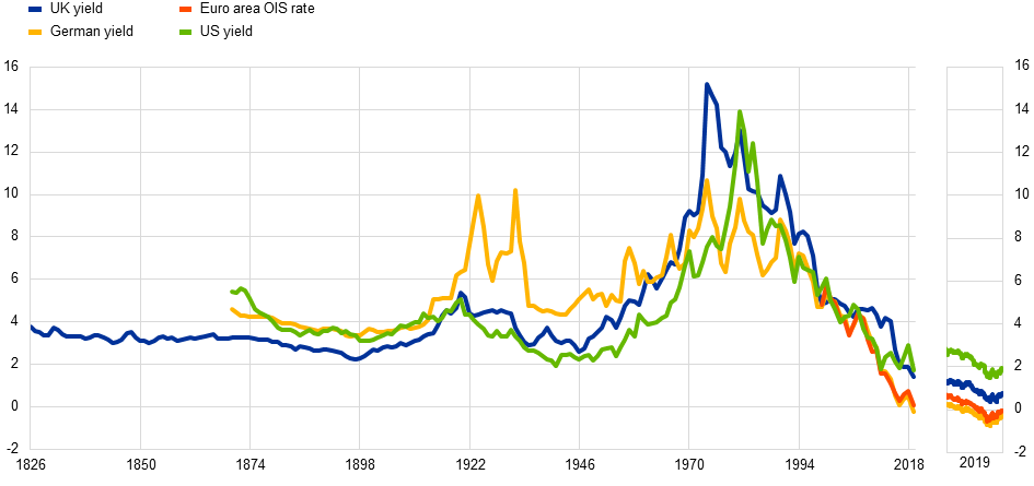
Sources: Bank of England, Bloomberg, FRED, Jordà et al. (2019), Thomson Reuters.
Notes: For the United Kingdom, the series is the rate on a consol, taken from the Bank of England data series “A Millennium of UK Data” (Thomas and Dimsdale, 2017). As of 2016, it is the yield of a 20-year zero coupon bond. For Germany, the series is the rate on a government bond or similar government debt instrument with 5-15 year maturity, derived from a variety of historical sources by Jordà et al. (2019). As of 1972, it is the ten-year German Bund rate. For the US, the series is the rate on government bonds with around ten-year maturity, provided by Jordà et al. (2019). As of 1960, it is the ten-year government bond rate. The euro area OIS rate is for ten-year maturity.Latest observation: 11 November 2019.
Yield curve slope and recessions in the euro area
(percentage points)
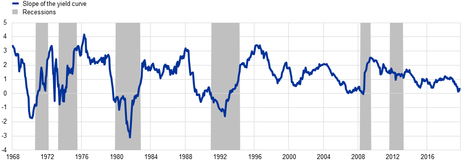
Sources: CEPR, OECD, ECRI, Bundesbank, Thomson Reuters and ECB calculations.
Notes: The slope of the yield curve shown is the spread between ten-year and one-year OIS yields since 1999. Before 1999, the spread is based on German bond data. German data back to 1972 are computed by the Bundesbank using the method of Svensson. German data prior to 1972 are extrapolated backwards based on historical series of short and long-term yields provided by the OECD. Long-term OECD yields refer to yields on outstanding listed federal securities with residual maturities of over nine to ten years traded on the secondary market. Short-term OECD yields are usually either the three-month interbank offered rates applicable to loans between banks, or the rates associated with Treasury bills, certificates of deposit or comparable instruments of three-month maturity in each case. Euro area (as of 1999) and German (before 1999) recessions are identified, respectively, by the CEPR and the Economic Cycle Research Institute (ECRI), with the exception of the German recession at the beginning of the 1970s identified by the OECD composite leading indicators.
Latest observation: October 2019.
At the same time, despite the unprecedented low level of the yield curve, the fact that the slope of the euro area yield curve is fairly flat (but slightly positive) is not at all unusual from a historical perspective (see Chart 2).[5]
The yield curve is a central element in the transmission of monetary policy. Standard and non-standard monetary policy instruments affect the whole of the term structure, which in turn is a key determinant of the financing conditions of the economy. Some rates in the euro area economy – such as corporate bond rates or mortgage loan rates – are based on longer-term risk-free yields, while others – such as bank loan rates for firms – are mostly priced off shorter maturities.[6] The financing conditions prevailing for firms and households in turn affect the level of economic activity and inflation.
While current monetary policy is an important factor affecting the yield curve, beliefs about future monetary policy and risk premia also play a role. In turn, these depend on a host of factors which determine the inflation or growth outlook of market participants and the evolution of risk premia. Accordingly, the yield curve plays a dual role for monetary policymakers: on the one hand, as a transmitter of monetary policy; on the other hand, as a source of information about the expectations and risk assessments of investors about the future macroeconomic environment and the future path for monetary policy.
Response of the yield curve to monetary policy in normal times
Let me first revisit the benchmark case of how the yield curve reacts to the standard policy tool of variations in short-term interest rates. To this end, I will focus on a rate cut, in order to facilitate the comparison with a subsequent discussion of our unconventional monetary easing policies.
When measuring the effect of monetary policy on the yield curve, macroeconomists typically focus on monetary policy shocks: that is, surprise changes in the policy rate that occur independently of other structural shocks, such as innovations in aggregate demand or cost-push shocks. Since monetary policy decisions respond to these other shocks, naive calculations of the co-variation between monetary policy and the yield curve cannot distinguish the contribution of monetary policy from the impact of the underlying structural shocks. Accordingly, the independent role of monetary policy is revealed by focusing on the surprise element in monetary policy decisions, and there is a buoyant literature trying to identify these shocks and measure their impact on the yield curve and the economy.
While earlier studies focused on the effect of contemporaneous rate surprises, more recent papers account for the fact that monetary policy decisions have typically been accompanied by explicit (or at least perceived) central bank communication on the future course of policy rates. Accordingly, the literature has started to distinguish between “rate surprises” and “path surprises” (or surprise changes to the forward guidance on future rates).[7] As was true for the earlier literature focusing on standard rate cuts, identification is a challenge: researchers need to separate rate surprises from path surprises and tell both apart from other structural shocks occurring at the same time.
Recent research involving ECB economists has used high-frequency movements in financial market variables to disentangle various types of monetary policy surprises affecting the yield curve during ECB press conferences: the impact of each type of surprise can be parsimoniously described by its “footprint” on the term structure (Chart 3).[8] A standard rate cut primarily affects the short end of the curve, while the impact peters out monotonically across the curve (Chart 3, left panel). By contrast, an innovation in the forward guidance on interest rates has a hump-shaped effect on the curve and exerts its maximum effect at a maturity of around two years (Chart 3, right panel).
Estimated effect of standard policy rate surprise (left-hand side) and rate path surprise (right-hand side) on the euro area OIS curve
(basis points)
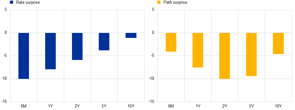
Sources: Based on Altavilla et al. (forthcoming).
Notes: The surprise impact is normalised to 10 basis points for the six-month (LHS) and two-year maturity (RHS), respectively.
An instructive way to rationalise those patterns is by reference to the expectations hypothesis of the term structure, according to which the long-term rate on a bond equals the average of short-term rates expected to prevail over the maturity of the bond. Under this assumption, a contemporaneous surprise in the short-term rate influences the short end of the curve one for one, while long rates will typically be affected less than one for one.[9] By comparison, a forward guidance surprise can be interpreted as leaving the current rate untouched while affecting the short-term interest rate path in the near and medium term. Taking an average over such an expected rate path gives rise to the observed hump-shaped footprint.
However, simple versions of the expectations hypothesis find little support in the data. Besides the average of expected short-term rates (the “expectations component”), long-term bond rates typically contain term premia, which are time-varying. In a nutshell, term premia are an average of expected excess returns over the lifetime of the bond, where the excess return measures the return from investing in a long-term bond over a short time period in excess of the risk-free short-term rate prevailing over that period.[10] Accordingly, term premia reflect both the riskiness of long-term bonds and the compensation required by investors for that risk. Abstracting from credit and liquidity risk, the most prevalent source of risk for long-term debt is duration risk: that is, the sensitivity of the bond price to changes in the yield curve. I will come back to this when discussing the duration channel of large-scale central bank asset purchases.[11]
Monetary policy exerts its effects on the yield curve not only through pure rate expectations but also through term premia. Chart 4 shows a model-based estimate of the yield curve response to a change in policy rates for the euro area.[12] The surprise used here is a combination of what I previously described as a pure rate surprise and a forward guidance surprise. It therefore affects yields across all maturities. While Chart 4 shows that changes in rate expectations explain the bulk of the yield curve response, part of it is attributable to changes in term premia.
Instantaneous impact of conventional policy surprise on expectations and term premia
(basis points)
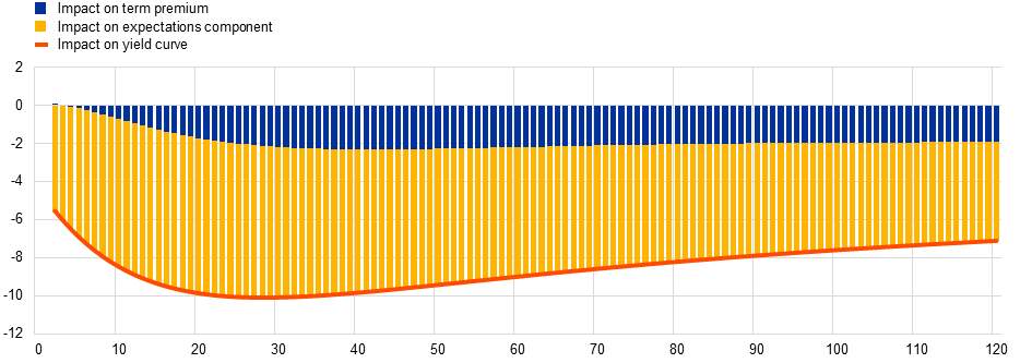
Source: ECB calculations.
Notes: The chart depicts the instantaneous impact of a conventional monetary policy surprise on the yield curve and its components. The policy surprise is identified through high-frequency changes in the common component of a set of euro area short-term interest rates of maturities up to one year. The surprise (normalised so that the one-month rate is reduced by 10 basis points) thus captures effects beyond a pure target rate surprise. These effects may be interpreted as a signalling element of conventional monetary policy. The impact is computed on the basis of a shadow-rate term structure model following Geiger and Schupp (2018). Estimates are based on a sample ending in June 2014 in order to avoid interference with the period of negative policy rates and asset purchases.
Some studies have looked at specific channels by which term premia help explain certain yield curve phenomena that can hardly be reconciled by the expectations hypothesis alone. For instance, Hanson and Stein (2015) observe that monetary policy rate decreases tend to coincide with surprisingly strong reactions in long-term forward rates.[13] One way to explain this pattern is by assuming that there may be “yield-oriented investors” in the market who do not trade based on forward-looking risk-return optimisation but rather react to changes in current yields. Those players may try to reallocate their portfolios in response to the policy-induced short rate decline in order to keep their average portfolio yields constant. Their increased demand for longer-term bonds will then increase bond prices and decrease term premia. This term premium compression will come on top of the decline in rate expectations and thus amplify the overall effect of a cut in short-term rates.
While this is one promising way to rationalise term premium responses to a monetary policy rate change, overall, our understanding of the interaction between monetary policy and term premia is still very limited. Take, for instance, the standard workhorse dynamic stochastic general equilibrium (DSGE) models commonly used by central bankers. Such models tend to abstract from the maturity structure of interest rates and the impact of term premia, especially in their commonly used linearised versions.
So far, we have seen the typical reaction of the yield curve to rate cuts in normal times: first, a reduction of the policy rate tends to lower and steepen the yield curve as short-term maturities decrease by more than their long-term counterparts; second, in addition to actual rate changes, communication about future rates influences the curve so that intermediate maturities react most strongly; and third, the transmission of monetary policy action and communication on short rates to long rates not only works through rate expectations but also through term premia.
Assessing the impact of non-standard monetary policy on the yield curve
The transmission of negative rates to the yield curve
Turning to non-standard policy, let me start with negative interest rates. Chart 5 shows the characteristic footprint of a cut in the policy rate – in negative territory – on the yield curve. It is constructed on the basis of high-frequency financial market information in the same way as Chart 3. There is a clear difference: compared with standard rate cuts in positive territory, rate cuts in negative territory have had a stronger effect further out along the yield curve.
Estimated effect of policy rate (deposit facility rate) cut in negative territory on the OIS curve
(basis points)

Sources: Based on Altavilla et al. (forthcoming).
Notes: Surprise impact normalised to 10 basis points for the six-month maturity.
Why do we see a stronger effect on longer maturities when the rate cut takes place in negative territory?
One factor here is that cuts in negative territory were often accompanied by communication or at least market perceptions that the ECB was willing to lower the negative rate even further, if warranted by subsequent economic conditions. As a case in point, for the final two of the last five rate cuts, the introductory statement at the press conference clarified that the ECB’s Governing Council “expects the key ECB interest rates to remain at present or lower levels”. This type of communication about the scope of negative rates can provide accommodation even in the absence of actual rate cuts. This mechanism adds another dimension to the standard channels of rate forward guidance.
Let me elaborate on this point. Consider the situation in which the central bank is perceived to be constrained by the zero lower bound. Guided by an understanding of the central bank’s reaction function and a depressed macroeconomic outlook, markets may think that in one year’s time, the central bank would like to set negative rates with positive probability but that, if constrained by the zero lower bound, the best the central bank can do in those states of the world is to keep rates at zero. In technical terms: the presence of the lower bound induces a censored distribution for future short rates. This in turn biases upwards the expectations of future short-term rates and hence steepens the whole term structure.[14] Communicating about a decrease in the lower bound makes rates possible that were previously perceived to be infeasible and, ceteris paribus, decreases expected future rates. By this reasoning, the lower bound itself – that is, the extent to which the central bank is willing to go negative if needed – becomes a policy parameter.[15]
Another potential way in which rate decreases in negative territory may have a more distinct effect is the accentuation of yield-seeking investor behaviour as in the Hanson-Stein setting that I described earlier. Those financial market participants that have a strong aversion to negative rates on short-term assets or an institutional need to avoid them altogether would seek to climb up the maturity ladder. This increased demand for longer-term debt would increase prices and decrease term premia. That is, the rate cut in negative territory would lead to a more accentuated search for yield that could amplify the yield curve reaction compared with what is observed on average in positive territory.
Through a similar mechanism negative rate policy can also be seen as complementary to our bond purchase programme (whose impact on the yield curve I will discuss in more detail later on).[16] In particular, the negative deposit rate reinforces the incentive of banks to actively seek higher-return alternatives rather than passively absorbing the excess liquidity created by quantitative easing.[17]
Finally, the negative interest rate policy also reinforces our targeted long-term refinancing operations (TLTROs).[18] Under the TLTROs, banks can refinance with the ECB at very favourable conditions: under the second and third wave of that programme (TLTRO II and III), borrowing rates in the TLTROs can be as low as the deposit facility rate (which is negative) if lending volume targets are met. Accordingly, the presence of negative rates provides a strong incentive for banks to participate in the TLTROs, which support credit provision to the real economy at attractive conditions.
The transmission of asset purchases to the yield curve
Let me now turn to large-scale asset purchases, including our own asset purchase programme (APP). There is a wide array of studies quantifying the effects of various forms of asset purchases on financial markets and macroeconomic variables. Results vary regarding the quantitative impact but there is a broad consensus that central bank asset purchases lead to a flattening of the curve, since the yields of longer-term bonds tend to decline by more than those of short-term bonds.
A first look at the stylised facts using the same approach that I outlined earlier confirms this pattern for the euro area. Extracting a quantitative easing factor from high-frequency interest rates and other financial market data confirms that news about ECB asset purchases had yield compression and flattening effects on the term structure, as shown in Chart 6.
Estimated effect of quantitative easing surprise on the OIS curve
(basis points)

Sources: Based on Altavilla et al. (forthcoming).
Notes: Surprise impact normalised to 10 basis points for the ten-year maturity.
The academic literature distinguishes broadly between two channels through which this policy works: signalling and portfolio rebalancing.[19]
Under the signalling channel, central bank asset purchases serve as a commitment device to keep policy rates at low levels for an extended period of time. Under the portfolio rebalancing channel, the central bank’s withdrawal of net bond supply from the market induces investors to reshuffle their portfolios, and these changes in demand-supply constellations affect bond prices and yields.
Under the signalling channel, the expectations component of bond yields decreases upon news about asset purchases, whereas under the portfolio rebalancing channel, the term premium component is compressed. The expectations and the term premium components cannot be observed separately. Econometric modelling is required to discriminate between the two components and provide a deeper understanding of the transmission channels of asset purchases.
An important episode studied by ECB researchers is the period before the announcement of the APP in January 2015. Between summer 2014 and the official announcement, some events reinforced the view of market participants that ECB government bond purchases were likely to start in the near future. The events examined by ECB staff occurred between the Governing Council meetings on 3 September 2014 and 22 January 2015, the day when the ECB announced the APP.[20] Cumulating across these events, the long-term Bund rate declined by 30 basis points. This is the bar that you see on the left in Chart 7. With the help of an econometric term structure model, ECB staff have decomposed that change into the contribution of changes in average short rate expectations and the term premium.[21] Chart 7 shows that it is the term premium that accounts for essentially the entire decline in yields. On the day of the APP announcement itself (22 January 2015), the ten-year Bund rate decreased by 15 basis points, which is one of the largest daily declines in Bund yields since the inception of the euro. The second bar in Chart 7 also shows that the observed yield compression can be explained exclusively by the term premium.[22]
Decomposed changes in ten-year Bund yields
(percentage points)

Sources: Based on Lemke and Werner (forthcoming).
Notes: Based on an affine term structure model, the bars shows the decomposed change of the ten-year Bund yield over the indicated horizons: left bar corresponds to cumulated one-day changes associated with APP-related ECB communication between summer 2014 and 22 January 2015. The other two bars correspond to a one-day change for the indicated date.
So staff analysis suggests that, at least initially, growing expectations of the imminent start of the APP were primarily reflected in a compression of the term premium.[23]
One way in which the portfolio rebalancing channel may affect bond yields is through a direct impact on demand and supply conditions in the maturity segment in which we purchase. For instance, buying a French eight-year bond decreases the supply of that bond available in the market. For given demand, this drives up the price of the bond and compresses its yield. Securities of similar maturity are close substitutes, so their yield would also be affected, but those with very short and much longer maturities would not be greatly affected. This is why this channel is often referred to as the “local supply channel”.
Another way in which the portfolio rebalancing channel is set in motion is through duration extraction.[24] The formalisation of this idea is based on prominent work by Vayanos and Vila (2009).[25] Let me just give you the basic mechanism. Going back to my previous example, under the duration extraction channel, the purchase of a French bond not only affects demand and supply locally but also reduces the aggregate risk to be borne by market participants. This leads price-sensitive investors to re-adjust their bond portfolio across maturities given their overall risk-bearing capacity. In terms of asset pricing terminology, central bank bond purchases decrease the market price of duration risk (the expected excess return on a long-term bond per unit of risk). As I explained earlier, excess returns constitute the term premium component of long-term bond yields, so term premia and overall bond yields decline.
An important implication of the duration channel is that it is not purchase flows that matter, but rather the stock of assets that the central bank is expected to hold on its balance sheet.[26] For instance, if the central bank announces a longer reinvestment horizon, it means that more duration risk is expected to be withdrawn from the market over a longer interval. The duration withdrawal leads to declining expected excess returns in the future. But those future excess returns are part of the current term premium embedded in a long-term bond. It follows that a longer reinvestment period in the future helps keep bond yields at low levels now.
Similar to analysis that accompanied the asset purchases of the Federal Reserve, ECB economists have quantified the effect of our asset purchases on the yield curve.[27] Based on a term structure model that incorporates the duration extraction channel that I just explained, Chart 8 shows estimates of how much the APP has compressed the yield curve in the euro area at different points in time.
APP impact on the euro area sovereign term structure
(basis points)
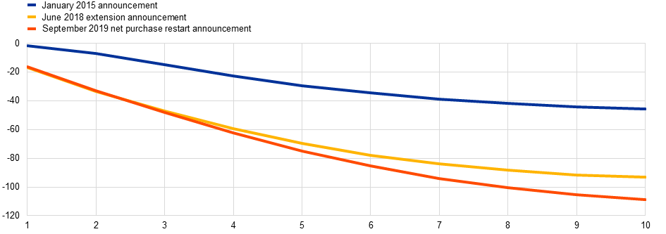
Sources: ECB, based on Eser et al. (2019).
Notes: The figure shows by how much the term premium component of euro area sovereign yields (weighted average of Germany, France, Italy and Spain) with maturities of one to ten years is estimated to be compressed due to the APP through the duration channel at three dates: the announcement of the APP (Jan 2015), the extension of the programme in June 2018, and the announcement of the restart of net purchases in September 2019.
APP impact on ten-year euro area sovereign yield over time
(basis points)

Sources: ECB, based on Eser et al. (2019).
Notes: Evolution of the APP impact on the ten-year synthetic sovereign yield (weighted average of Germany, France, Italy, Spain). The impact is derived on the basis of an arbitrage-free affine model of the term structure with a quantity factor (see Eser et al. 2019).
Latest observation: September 2019.
The first point is January 2015 when the ECB had just announced that it would start purchases in the following March at a rate of €60 billion per month, intended to run until September of the following year. According to ECB staff estimates, the anticipation of the purchases, the associated balance sheet accumulation of the ECB and, as a flip side of the coin, the expected duration extraction were associated with a term premium compression of almost 50 basis points for the ten-year maturity. For shorter-term bonds the effects are lower, such that the expectation of asset purchases is estimated to have led to a flattening of the curve. Moreover, by virtue of the stock effect, the yield compression was expected to be long-lasting and to halve only after five years.
Owing to changes in macroeconomic conditions and the need to adapt the monetary policy response, several recalibrations were made to the APP.[28] Accordingly, as is shown in Chart 9, the contemporaneous term premium impact changed over time, reaching its maximum of more than 100 basis points in mid-2016, when markets were expecting a significant expansion of the APP in light of increased uncertainty induced by the Brexit referendum outcome. When the end of net purchases was announced in June 2018, the impact on ten-year sovereign bond yields was estimated to be around 90 basis points. The additional duration extraction associated with the renewed net purchases that started this month has contributed to a further compression of the term premium. Currently, staff estimate the euro area sovereign ten-year rate to be more than 100 basis points lower than in a counterfactual where the APP never happened, and the curve to be distinctly flatter (see again Chart 8).
Finally, there are also complementarities between the APP and other instruments, which I will briefly summarise.[29] First, the APP helps maintain the excess liquidity conditions that keep the euro short-term rate (€STR), the interbank overnight rate in the euro area, near the ECB’s deposit facility rate, which in turn contributes to avoiding undesirable bouts of interest rate volatility. Second, as an immediate consequence of the induced tight link between the deposit facility rate and the €STR, our forward guidance on the official ECB rate will effectively be mapped directly onto expectations of the market-relevant €STR. And third, capital gains for bond-holding banks can free up balance sheet capacity that banks can redeploy to generate commercial loans under the TLTRO scheme.
Summary of the yield curve effects of the ECB’s non-standard policies
Putting several pieces of analysis together, ECB economists have come up with the following summary assessment of how the various non-standard policy measures since 2014 have affected the yield curve.
Compression of euro area sovereign yield curve due to ECB’s non-standard measures
(percentage points)

Sources: Based on Rostagno et al. (2019).
Notes: The chart illustrates the contribution of individual measures. The results are based on a Bayesian vector auto-regression. The impact of NIRP (negative interest rate policy) and FG (forward guidance) on sovereign yields works via the short-term rate and the OIS forward curve, and the impact of the APP operates via term premia.
As we see in Chart 10, covering the annual averages from 2014 to 2018, the APP accounted for the bulk of the estimated yield compression at the long end of the curve. Negative interest rates and forward guidance, by contrast, account for the lion’s share at the short end of the curve. Overall, taking the APP, negative rates and rate forward guidance together, ten-year sovereign bond yields would have been almost 1.4 percentage points higher in 2018 without those measures. These yield compressions have been transmitted further to an easing of financing conditions for non-financial corporations and households.[30]
Interpreting signals from a flattening curve under central bank asset purchases
The significant effect that our monetary policy had on the yield curve helped to improve financing conditions and ease the monetary policy stance. At the same time, the strong impact of our own policy makes it more difficult to read the information that the yield curve may incorporate regarding the outlook for the economy. An important and currently relevant example is the question as to what extent a flattening yield curve signals a weakening of the economic outlook.
There has been a considerable body of literature devoted to this question. An important strand focuses on the negative correlation between the slope of the yield curve and the probability of future recessions, and the possible economic mechanisms underlying such a pattern. I will just briefly highlight how important it is to take our own action into account when interpreting the signals reflected in the yield curve.
For the euro area, and for Germany over earlier years, we see indeed the regularity that recessions tend to have been preceded by a flattening yield curve (see Chart 2 again). A recent paper examines how economists and commentators, when confronted with a flattening curve in the past, often argued that “this time is different”.[31] That is, they claimed that special factors were contributing to the flatter curve and that these compromised the standard interpretation of the curve as a harbinger of recession.
As I mentioned at the beginning, the current euro area yield curve is indeed quite flat from a historical perspective, with the spread between ten-year and one-year yields amounting to about 30 basis points, which is around 1 percentage point lower than on average.[32] I will certainly not make a binary statement on whether this time is different. In particular, a sound assessment of the future growth outlook should be based on a wide range of indicators and models, rather than the yield curve alone. Moreover, there are two further issues to consider.
First, the current flattening of the curve has mainly been induced by the long end of the curve coming down, rather than by the short end coming up. This constellation is different from previous episodes of yield curve inversion, as is shown in Chart 11. Hence, the inversion of the yield curve observed this time is not occurring in a context of monetary policy contraction raising the short end of the curve.
Decomposition of change in the slope of the yield curve
(percentage points)
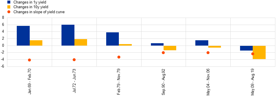
Sources: Bundesbank, OECD, Thomson Reuters and ECB calculations.
Notes: Update of the corresponding chart in De Backer et al. (2019). The changes in the slope of the yield curve are calculated from peak to trough. See the footnote of Chart 2 for more details regarding the underlying data.
APP impact on the euro area OIS curve
(percent per annum)
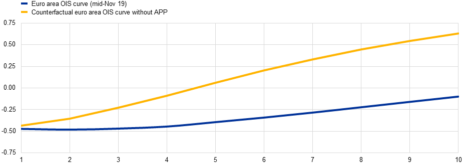
Sources: ECB, based on Eser et al. (2019).
Notes: The blue line represents the overnight index swap (OIS) curve as of mid-November 2019. The yellow line represents an estimate of the corresponding counterfactual curve that would have prevailed in the absence of the APP.
Second, the flattening of the curve is to some extent driven by our own asset purchases conducted for the purpose of stimulating the economy. As is shown in Chart 12, one observes that the current slope would be around 70 basis points higher in the absence of the APP and thus much closer to the historical average.[33]
What we learn from this example is that we need to be careful when reading the yield curve especially during times when our own actions have a significant influence on it. Despite this caveat, we pay careful attention to the evolution of the yield curve, in order to assess the views of investors concerning future macroeconomic and policy developments and explore non-monetary factors that can influence term premia, such as global shifts in portfolio preferences, risk distributions and risk-absorbing capacity.
Conclusion
Let me conclude. The yield curve plays a key role for the transmission of monetary policy, under both standard and non-standard policy measures. Our non-standard measures of negative interest rate policy and asset purchases brought down the overall level of the yield curve to a region that is, by definition, unreachable under a zero lower bound and contributed to a considerable flattening of the term structure. The lowering and flattening of the yield curve in turn eased financing conditions for non-financial corporations and households, contributed to spurring economic activity and helped bring inflation closer towards our aim.
From an analytical perspective, further study of the impact of innovative monetary policy measures is a necessity for central bankers and an opportunity for academics. While academic researchers have the privilege of being able to watch new policy measures unfold before scrutinising their impact, central bank researchers and decision-makers have to monitor the impact of policy in real time, and are forced to rely on sparse empirical evidence, especially if the policy measure is unprecedented.
There are many open issues regarding the interplay between the yield curve and monetary policy that require further research in my view. So let me finish with a little wish list or research agenda. First on the list should be a better understanding of the role of term premia in macroeconomic models. This includes a more thorough analysis of the transmission of quantitative easing through the duration channel, but also, more generally, a better integration of long-term rates in the transmission mechanism as formalised in DSGE models. [34] Second is an improved modelling of long-term trends. Both the macro and the asset pricing literature seem to have understood the importance of taking time-varying long-run equilibria into account, but a coherent treatment within macro finance models would be desirable.[35] And a third theme is an improved modelling of cross-country interrelations: this pertains to a more refined understanding of the workings of quantitative easing in a currency union, but also to the spillovers of policy-induced yield curve changes across different currency areas.[36],[37] Finally, one question is whether changes in long-term rates that are due to changes in the risk-less rate versus the term premium have similar effects on spending and the economy.
On these and other topics concerning the interplay between monetary policy and the yield curve, I look forward to learning from new academic research – including the future contributions of the UCL research community. Thank you for your attention.
- [1]I am grateful to Wolfgang Lemke for his contribution to this speech.
- [2]On how to measure the risk-free rate in the euro area appropriately, see European Central Bank (2014), “Euro area risk-free interest rates: measurement issues, recent developments and relevance to monetary policy”, Monthly Bulletin July.
- [3]Some of the long time series shown in Chart 1 are from Jordà, Ò., Knoll, K., Kuvshinov, D., Schularick, M. and Taylor, A. M. (2019), “The rate of return on everything, 1870–2015”, The Quarterly Journal of Economics, 134(3), pp. 1225-1298.
- [4]Today, I will not discuss the potential non-policy drivers of the secular downward trend in rates that I mentioned earlier. This is an important discussion, in which the decline of the natural real rate of interest plays a central role. Its measurement, an understanding of its drivers and its relevance to monetary policy are crucial issues that are in the spotlight of academic research and central bank discussions. See, amongst others, Brand, C., Bielecki, M. and Penalver, A. (2018), “The natural rate of interest: estimates, drivers, and challenges to monetary policy”, Occasional Paper Series, No 217, ECB; Bauer, M. D. and Rudebusch, G. D. (2019), “Interest Rates Under Falling Stars”, Federal Reserve Bank of San Francisco Working Paper 2017-16; Kiley, M. T. (2019), "The Global Equilibrium Real Interest Rate: Concepts, Estimates, and Challenges", Finance and Economics Discussion Series 2019-076, Board of Governors of the Federal Reserve System; and Clarida, R. H. (2019), “Monetary Policy, Price Stability, and Equilibrium Bond Yields: Success and Consequences”, Speech at the High-Level Conference on Global Risk, Uncertainty, and Volatility, Zurich, 12 November. I will discuss the drivers of the low level of rates in another speech later this week.
- [5]Modelling and interpreting the level and the shape of the yield curve is an active field of research. Since Irving Fisher’s “Appreciation and Interest” and John Hicks’s “Value and Capital”, which are sometimes referenced as the earliest formalisations of the expectations hypothesis of the term structure, hundreds of research papers on the joint dynamics of bond yields of different maturities have been produced. This work spans (i) purely econometric studies trying to capture salient time series features of term structure dynamics; (ii) a rich finance literature studying the pricing of bonds and interest rate derivatives in a no-arbitrage framework; and (iii) a host of reduced-form or structural models trying to link the yield curve to macroeconomic variables. Traditionally, and especially recently, central bank economists have been quite active in that type of research.
- [6]See Darracq Pariès, M., Moccero, D., Krylova, E. and Marchini, C. (2014), “The retail bank interest rate pass-through: the case of the euro area during the financial and sovereign debt crisis”, Occasional Paper, No 155, ECB; and European Central Bank (2017), “MFI lending rates: pass-through in the time of non-standard monetary policy”, Economic Bulletin, Issue 1.
- [7]See Gürkaynak, R., Sack, B. and Swanson, E. (2005), “Do Actions Speak Louder Than Words? The Response of Asset Prices to Monetary Policy Actions and Statements”, International Journal of Central Banking, 1(1), pp. 55-93.
- [8]See, e.g., Altavilla, C., Brugnolini, L., Gürkaynak, R. S., Motto, R. and Ragusa, G. (forthcoming), “Measuring euro area monetary policy”, Journal of Monetary Economics. For similar approaches, see also Cieslak, A. and Schrimpf, A. (forthcoming), “Non-Monetary News in Central Bank Communication”, Journal of International Economics; and Leombroni, M., Vedolin, A., Venter, G. and Whelan, P. (2018), “Central Bank Communication and the Yield Curve”, CEPR Discussion Papier 12970.
- [9]As a general pattern stipulated in most models, the short-term rate is typically expected to revert back to some long-term mean. With (changes in) long rates being equal to (changes in) average short rates under the expectations hypothesis, the contemporaneous impact on the long rate thus depends on the persistence of the short rate.
- [10]See, e.g., Cochrane, J. H. and Piazzesi, M. (2008), “Decomposing the Yield Curve”, Working Paper, University of Chicago.
- [11]It is important to keep in mind that term premia are not directly observable: decomposing observed bond yields into the expectations component and term premia requires econometric modelling, which is subject to considerable estimation and model uncertainty. For an overview see Cohen, B., Hördahl, P. and Xia, D. (2018), “Term premia: models and some stylised facts”, BIS Quarterly Review, September, pp. 79-90. Most recently, researchers have highlighted that the level and dynamics of estimated term premia depend considerably on how the long-horizon expectation of short-term rates is modelled: linking those future end-points to the time-varying levels of the natural rate gives rise to term premia that display less of a trend decline than those from commonly used models with a time-constant equilibrium rate, see Bauer and Rudebusch (2019) op. cit. Recent research by ECB economists on the euro area finds similar evidence.
- [12]The exercise is based on the model by Geiger, F. and Schupp, F. (2018), “With a little help from my friends: Survey-based derivation of euro area short rate expectations at the effective lower bound”, Bundesbank Discussion Paper, No 27.
- [13]Hanson, S. G. and Stein, J. C. (2015), “Monetary Policy and Long-Term Real Rates”, Journal of Financial Economics, 115(3), pp. 429-448.
- [14]See Ruge-Murcia, F.-J. (2006), “The expectations hypothesis of the term structure when interest rates are close to zero”, Journal of Monetary Economics, 53, pp. 1409-1424.
- [15]See Lemke, W. and Vladu, A. (2017), “Below the zero lower bound: a shadow-rate term structure model for the euro area”, Working Paper Series, No 1991, ECB; Rostagno, M., Altavilla, C., Carboni, C., Lemke, W., Motto, R., Saint-Guilhem, A., Yiangou, J. (2019), “A Tale of Two Decades: the ECB’s Monetary Policy at 20”, ECB mimeo; and Bottero, M., Minoiu, C., Peydro, J.-L., Polo, A, Presbitero, A., Sette, E. (2019), “Negative Monetary Policy Rates and Portfolio Rebalancing: Evidence from Credit Register Data”, IMF Working Paper 19/44 and Wu, C., Xia, D., (2018), “Negative Interest Rate Policy and the Yield Curve”, NBER Working Paper W25180.
- [16]For a summary of the potential complementarities between negative rate policy, forward guidance, asset purchases and TLTROs see the respective matrix in Chapter 6 of Rostagno et al. (2019), op. cit.
- [17]See, for example, Ryan and Whelan (2019), “Quantitative Easing and the Hot Potato Effect: Evidence from Euro Area Banks”, Research Technical Paper, Central Bank of Ireland, Vol. 2019, No 1 on the hot potato effect.
- [18]For an overview on the working of TLTRO, see European Central Bank (2017), “The targeted longer-term refinancing operations: an overview of the take-up and their impact on bank Intermediation”, Box in Economic Bulletin, Issue 3.
- [19]See, e.g., Bauer, M. D. and Rudebusch, G. D. (2014), “The Signalling Channel for Federal Reserve Bond Purchases”, International Journal of Central Banking, 10(3), pp. 233–290. See also Broadbent, B. (2018), “The history and future of QE”, Speech given at Society of Professional Economists, London, 23 July 2018, and Christensen, J. and Krogstrup, S. (forthcoming), “Transmission of Quantitative Easing: The Role of Central Bank Reserves”, Economic Journal, who argue for another channel emphasising the relevance of reserves for the balance sheets of commercial banks.
- [20]In addition to the press conferences following Governing Council meetings the events also include other public communication by ECB President Mario Draghi. At the press conference following the September 2014 Governing Council meeting, the first in the event cluster, the President explicitly answered a journalist’s question with the words “Yes, it was discussed. QE was discussed. […]. A broad asset purchase programme was discussed, and some Governors made clear that they would like to do more”.
- [21]See Lemke, W. and Werner, T. (forthcoming), “Dissecting long-term Bund yields in the run-up to the ECB’s public sector purchase programme”, Journal of Banking and Finance.
- [22]At the same time, the dominating role of the term premium is not a general feature or model artefact. As exemplified by the right-hand bar in Chart 7, there are events where rate expectations are the dominating factor. The particular date shown there corresponds to an ECB press conference during the financial crisis that induced market participants to adjust markedly their policy rate expectations.
- [23]This result is qualitatively in line with Joyce, M., Tong, M. and Woods, R. (2011), “The United Kingdom’s quantitative easing policy: design, operation and impact”, Bank of England Quarterly Bulletin 2011Q3 who find that “the fall in gilt yields cannot primarily be attributed to signalling effects […] Instead, it is consistent with the main effect coming through portfolio rebalancing”. Bauer and Rudebusch (2014), op. cit., by contrast, find up to one half of the US LSAP effects on yields coming through signalling, challenging earlier literature giving less weight to this channel. In addition, Broadbent (2018) op. cit. argues that the effects of asset purchases and the relative importance of the channels through which they work can vary over time.
- [24]Duration extraction was highlighted also as a prominent channel for the Federal Reserve’s LSAP, see the seminal paper by Gagnon, J., Raskin, M., Remache, J. and Sack, B. (2011), “The Financial Market Effects of the Federal Reserve’s Large-Scale Asset Purchases”, International Journal of Central Banking, 7(1), pp. 3-43, which stresses exactly the type of mechanism that ECB staff tried to quantify for the euro area: “The LSAPs have removed a considerable amount of assets with high duration from the markets. With less duration risk to hold in the aggregate, the market should require a lower premium to hold that risk. This effect may arise because those investors most willing to bear the risk are the ones left holding it. Or, even if investors do not differ greatly in their attitudes toward duration risk, they may require lower compensation for holding duration risk when they have smaller amounts of it in their portfolios.”
- [25]Vayanos, D. and Vila, J. (2009), “A preferred-habitat model of the term structure of interest rates”, NBER Working Paper, No 15487.
- [26]For the euro area, flow effects are found to be small, yet sometimes significant, see, e.g., the overview in Arrata, W. and Nguyen, B. (2017), “Price impact of bond supply shocks: Evidence from the Eurosystem’s asset purchase program”, Banque de France Working Paper, No 623; as well as De Santis, R. and Holm-Hadulla, F. (2017), “Flow effects of central bank asset purchases on euro area sovereign bond yields: evidence from a natural experiment”, Working Paper Series, No 2052, ECB; or Schlepper, K., Ryordan, R., Hofer, H., and Schrimpf, A. (2017), “Scarcity effects of QE: a transaction-level analysis in the Bund market”, Deutsche Bundesbank Discussion Paper, 06/2017.
- [27]For quantifying the yield curve impact via the duration channel in the United States and the euro area, see respectively Li, C. and Wei, M. (2013), “Term structure modelling with supply factors and the Federal Reserve’s large-scale asset purchase programs”, International Journal of Central Banking, 9(1), pp. 3–39; and Eser, F., Lemke, W., Nyholm, K., Radde, S. and Vladu, A. (2019), “Tracing the impact of the ECB’s asset purchase programme on the yield curve”, Working Paper Series, No 2293, ECB.
- [28]See, e.g., Hammermann, F., Leonard, K., Nardelli, S. and von Landesberger, J. (2019), “Taking stock of the Eurosystem’s asset purchase programme after the end of net asset purchases”, Economic Bulletin, Issue 2, ECB; and Rostagno et al. (2019), op. cit.
- [29]See again the respective matrix in Rostagno et al. (2019), op. cit.
- [30]See Hammermann et al. (2019), op. cit.
- [31]See De Backer, B., Deroose, M. and Van Nieuwenhuyze, Ch. (2019), “Is a recession imminent? The signal of the yield curve”, NBB Economic Review, June, pp. 69-93.
- [32]The choice of that particular spread (as opposed to the commonly used one-year minus thee-month) follows De Backer et al. (2019), op. cit.
- [33]The effect on the slope of the OIS curve is about two-thirds of the effect on the sovereign bond curve reported before.
- [34]See, e.g., King, T. B. (2018), “Duration Effects in Macro-Finance Models of the Term Structure”, mimeo.
- [35]This mirrors the postulation in a recent paper on the natural real rate by Kiley (2019), op. cit., stating the “need for further integration of financial and macroeconomic approaches to understanding trends in interest rates”.
- [36]See, e.g., Bletzinger, T. and von Thadden, L. (2018), “Designing QE in a fiscally sound monetary union”, Working Paper Series, No 2156, ECB.
- [37]See, e.g., Curcuru, S. Kamin, S., Li, C. and Rodriguez, M. (2018), “International Spillovers of Monetary Policy: Conventional Policy vs. Quantitative Easing”, Federal Reserve Board of Governors, International Finance Discussion Papers, No 1234.
European Central Bank
Directorate General Communications
- Sonnemannstrasse 20
- 60314 Frankfurt am Main, Germany
- +49 69 1344 7455
- media@ecb.europa.eu
Reproduction is permitted provided that the source is acknowledged.
Media contacts